This step-by-step procedure aims to illustrate how to develop a burn severity map in order to assess areas affected by wildfires. The Normalized Burn Ratio (NBR) is used during the process as it highlights burned areas in large fire zones. After creating the pre-fire and post-fire NBR images, the post-fire image is subtracted from the pre-fire image to create a differenced (or delta) NBR (dNBR) image. dNBR can then be used for burn severity assessment after being classified according to the burn severity ranges proposed by United States Geological Survey (USGS).
Data required during this practice:
- Landsat 8 pre-fire NIR and SWIR2 images
- Landsat 8 post-fire NIR and SWIR2 images
- Shapefile of Empedrado area, Chile
- QGIS Software
To follow the step by step on how to DOWNLOAD the data for this practice, please click here.
This procedure was developed using QGIS Las Palmas version 2.18.3. QGIS can be downloaded here.
Content
QGIS basics
Data Preparation/Pre-processing
Step 1: Open Images in QGIS
Step 2: Top of the Atmosphere (TOA) corrections
Processing Steps
Step 3: Calculating the Normalized Burn Ratio (NBR)
Step 4: Calculating delta NBR (dNBR)
Step 5: Clipping the image
Assessment
Step 6: Setting the ranges according to USGS standard
Step 7: Area Calculation
Additional: Composition of the map
QGIS basics
QGIS is an Open Source Geographic Information System (GIS) licensed under the GNU General Public License. QGIS is an official project of the Open Source Geospatial Foundation (OSGeo). It runs on Linux, Unix, Mac OSX, Windows and Android and supports numerous vector, raster, and database formats and functionalities (QGIS).
To start working, open the QGIS Desktop. Figure 1 illustrates an example of the QGIS Desktop interface, the Browser and Layers Panels and the Map Canvas. The QGIS Browser is a panel from which you can access your database. In the Layers Panel, there is a list of all the layers that you have added to your map. You can also expand collapsed items (by clicking the arrow or plus symbol beside them). This will provide you with more information on the layer’s current appearance.

Figure 1. QGIS interface.
Burn Severity
To start processing, you should have already downloaded the relevant images and shapefile of the study area. The files that you should have to start processing are listed below. If you have not downloaded them yet, please click here.
- The folder containing pre-fire images (for this procedure, the Landsat 8 images name used for pre fire is LC80010852017008LGN00);
- The folder containing post-fire images (for this procedure, the Landsat 8 images name used for pre fire is LC80010852017056LGN00);
- The shapefile of the assessed area (under the name Empedrado).
1. Open Images in QGIS
There are two ways you can open the downloaded images in QGIS. One way is using the browser panel (explained in section a), and the other way would be using menu toolbar (explained in section b). You can choose which way is more suitable for you.
The layers that will be added were acquired by Landsat8 before and after the fire. The bands that will be used to calculate the Normalized Burn Ration (NBR) are the Near Infrared (NIR) and Shortwave Infrared-2 (SWIR2), which correspond to band 5 and band 7, respectively. More about NBR, please click here.
The layers you should add at the moment should be:

a. Opening images using the browser panel
Please find where you have stored your images, select the bands that are going to be used for NBR. Once each layer has been selected, double-click it to add it to the Map Canvas or you can also drag-and-drop the layer to the Map Canvas (Figure 2).

Figure 2. Opening images using the browser panel in QGIS.
b. Opening images using the menu toolbar
To open the images using the menu toolbar, please click on Layer -> Add Layer -> Add Raster Layer (Figure 3). This should open a window where you can find the folder where the bands are stored. When you find them, select and click open for each of the bands.

Figure 3. Opening images using the menu toolbar in QGIS.
After the images are loaded into Map Canvas, you should see them on the layers panel, as indicated by the red box in Figure 4.

Figure 4. Screenshot demonstrating how the Layers Panel should look after loading the relevant bands.
2. Top of the Atmosphere (TOA) corrections
In order to calculate NBR, it is recommended to correct the images for the TOA reflectance.
2.1. Installing the Semi Automatic Classification Plugin
Firstly, please be sure that you have administrator rights on your computer, i.e. that you are authorized to install software and plugins. For this procedure, you will be required to install a plugin.
To correct for the TOA in QGIS, the Semi Automatic Classification plugin is used. So before correcting, please be sure that you have the plugin installed. To install it, please go to Plugins -> Manage and install plugins… (Figure 5).

Figure 5. Screenshot indicating where to install plugins from the menu toolbar (red box).
After clicking on Manage and Install Plugins… a new window should open where you can search for plugins to be installed. Please type on the search box 'Semi-Automatic'; after typing it should automatically show you the plugins options that correspond to the search (Figure 6). After selecting the Semi-Automatic Classification (SCP) Plugin, please click install on the bottom right corner of the window (indicated by the red box in Figure 6).

Figure 6. Plugins' search in QGIS.
2.2. Open the SCP pre-processing window
So now there should be SCP icon on your menu toolbar. Please go to SCP -> Preprocessing -> Landsat, as demonstrated in the red box in Figure 8. You can see that after the plugin has been installed, a new window could open on the bottom left corner, indicated in green in Figure 7. The SCP dock provides a quick access to some of the SCP plugin’s functions.

Figure 7. Screenshot demonstrating the path to follow (red box) and the SCP dock (green box).
After following the path and clicking Landsat, a new window should open, such as the one shown in Figure 8. Click on the yellow icon indicated by a red box in Figure 8 to select the folder where your images and metadata are. It is important that the folder structure remains the same as downloaded because the plugin will automatically use the correspondent metadata.

Figure 8. Semi-Automatic Classification Plugin window.
2.3. Select the folder that contains the pre-fire images
After selecting the folder that contains the pre-fire images, you should see your folder path on the 'Directory containing Landsat bands'. The bands that are in the selected folder are shown (red box in Figure 9) You should also see the metadata automatically loaded, showing the satellite, image date, sun elevation and Earth sun distance (top of the red box in Figure 9).
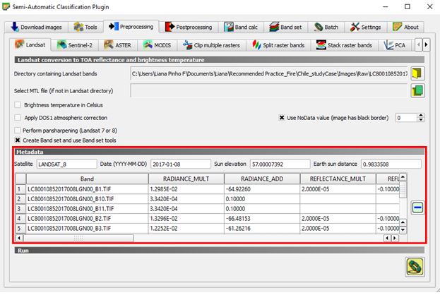
Figure 9. Semi-Automatic Classification Plugin window after selecting the folder with Landsat 8 pre-fire images.
2.4. Top of Atmosphere (TOA) corrections
On the SCP processing window, please select Apply DOS1 atmospheric corrections. This option will not correct the thermal bands. Leave both Create Band set and use Band set tools and Use NoData value (image has black border) options selected. Please remove the bands that will not be used during the NBR process, i.e. remove all bands except bands 5 and 7 (Figure 10). This way, the corrections will only be performed on the relevant layers, which will improve the computing time. Please select the layers you would like to remove and click on the 'minus' icon on the right-hand side. Your SCP window should then look similar to the one in Figure 10.
TIP: You can select multiple files to be removed by holding the Ctrl key on your keyboard while selecting the files.

Figure 10. SCP window showing the bands to be corrected.
Please note that after clicking run, it will ask you to select the folder where the corrected images will be stored. In case you do not already have a folder created, simply click on create folder to create a new one (Figure 11).

Figure 11. Screenshot showing the icon to create a new folder to store the corrected images.
This process could take a few minutes depending on the computer’s configuration. The progress can be monitored in the main window of QGIS, where a progress bar is shown.
Please note that the corrected bands are automatically added to the layers panel, with 'RT' in front of the file name.
Now, the pre-fire images have already been corrected, however the post-fire images still need to be processed for the TOA corrections. Please also correct the post-fire images following the same steps as the ones gone through for the pre-fire images, i.e. from step 2.3.
After having the pre and post-fire images corrected, your QGIS should be looking similar to the one shown in Figure 12.

Figure 12. Screenshot of the processing done until now.
- IN THE FOLLOWING STEPS, ONLY THE CORRECTED IMAGES WILL BE USED.
3. Calculating the Normalized Burn Ratio (NBR)
NBR is calculated using the NIR and SWIR2 bands from Landsat 8 during this practice, as shown in the formula below. If you would like to know more about NBR, please click here.
NBR = (NIR – SWIR2) / (NIR + SWIR2)
In order to calculate NBR in QGIS, the tool Band Calc will be used. So please go to SCP -> Band Calc. After selecting the Band Calc tool, it should open a new window, as indicated by the red box in Figure 13.

Figure 13. Screenshot demonstrating the Band Calc tool.
To assess burn severity, NBR should be calculated for both pre and post-fire images. This will then enable the calculation of their difference (dNBR) and burn severity.
3.1. Calculate pre-fire NBR
First of all, after the Band Calc window is open, press the refresh list button on the right side ( ). This will update the list of raster files available for calculation. Then, enter the following expression to calculate NBR for the pre-fire images:
TIP: To add the files that will be used in the expression, you can simply double click on their names and it will add them to the expression.

Figure 14. Screenshot of the expression for the NBR calculation.
After inserting the expression, click Run (icon in the bottom right corner, indicated in Figure 14). After clicking Run, you will be able to select which folder you would like to save the new file and you can name the file as you prefer. During this procedure, it was named as Pre_NBR.

Figure 15. Screenshot of the processing done after running the post-fire NBR.
4. Calculating delta NBR (dNBR)
After calculating NBR for both pre and post-fire images, it is possible to determine their difference and obtain dNBR. Therefore, first, you should calculate the difference between the NBR before and after the fire, referred to as dNBR during this practice. For that, the NBR of the post-images is subtracted from the NBR of the pre-images, as shown in the formula below:
dNBR = pre-fire NBR – post-fire NBR
Open the Band Calc tool again (SCP -> Band Calc) and click the refresh list icon again, so the new calculated files will also appear. Remove the previous expression and insert the following one:
After clicking Run, please select the folder where you would like the new file to be added into and the name of the file. The calculated dNBR should be added automatically to the Layers Panel and Map Canvas. By now, you should be seeing a similar screen as the one shown in Figure 16.

Figure 16. Screenshot of the processing done after running dNBR.
5. Clipping the image
The shapefile of the correspondent area (i.e. Empedrado) will be used to clip the raster dNBR to obtain an image reflecting only the study area. As during this recommended practice, we are using the area of Empedrado region in Chile, the administrative boundary of the aforementioned area will be used. If you have not downloaded Empedrado’s shapefile yet, please click here for instructions.
5.1. Adding the shapefile
To crop the image, find the 'Empedrado' shapefile through the Browser Panel and add it to the Map Canvas. How to add was described on the first step of the Image Processing section. After adding the shapefile, you should see the shapefile on top of your images, as it can be seen in Figure 17. Please note that the shapefile color shown may differ, as it is automatically selected by QGIS.
5.2. Clipping dNBR
To crop the image, please go through the menu toolbar and click Raster -> Extraction -> Clipper (Figure 17) and the Clipper dialog window should automatically open.

Figure 17. Screenshot of QGIS window demonstrating how to open the Clipper dialog.
In the Clipper dialog, select the dNBR raster as the Input file. Then, click on 'Select…' to set the name and address path for the output file. In the 'Clipping mode section', it is important to select the Mask layer mode. This will enable you to select the shapefile that you would like to use to clip the raster. Then, select 'Empedrado' shapefile as the Mask layer. Also, it is convenient to have the box for 'Load into canvas when finished' checked. This will load the clipped raster automatically when it is finished processing. The Clipper dialog box is illustrated in Figure 18. When everything is checked, click 'OK'.

Figure 18. Clipper dialog window illustrating the options that should be selected to clip dNBR.
After clipping, the raster showing only the Empedrado area is automatically loaded into the Layers Panel and Map Canvas. In order to see only the study area in Map Canvas, deselect the other raster files in the Layers Panel, leaving only the clipped raster selected. After that, you should be seing the clipped area on your Canvas.
The raster shown displays the image stretching based on the histogram statistics calculated for the entire image. In order to stretch the image based on the statistics calculated only for the portion of the image displayed, please right click on the correspondent image name on Layers Panel and choose Stretch Using Current Extent. After clicking on it, you should see a change in the highest and lowest pixel values. You should also see the raster as it is shown in Figure 19.

Figure 19. Screenshot after stretching the raster using the current extent.
6. Setting the ranges according to USGS standard
USGS standard will be used to classify the burn severity map according to the proposed number ranges, as explained here.
6.1. Classifying dNBR
To classify the map, right click the file name under the Layers Panel and select Properties.
After clicking properties, the 'Layer Properties' dialog should open in a new window. Please select the tab called Style. In this tab, please change the features as demonstrated below:
- Change the Render type to Singleband Pseudocolor;
- Change the Mode to Equal interval;
- Change Classes to 10.
You should see the amount of classes automatically increasing in the central viewer (Figure 20)

Figure 20. Layer Properties dialog window.
Now we will change the values (according to USGS standard) and colors of the Layer Properties. The upper and lower boundaries will be introduced separately. Please fill out the ranges to match the Layer Properties dialog shown in Figure 21, which is based on the table shown here. The choice of colors is not standardize and therefore, it is up to the user to choose the color palette.
Please note: The boundaries for the highest and lowest value for burn severity is set by the values on the image. For example, the lowest value on the map is -0.0594, demonstrating that there were no values related to regrowth. The legend will only reflect the classes available on the map.

Figure 21. Screenshot of the ranges used for classification.
After inserting the ranges, click Apply and OK. You should then see a similar map to the one in Figure 22.
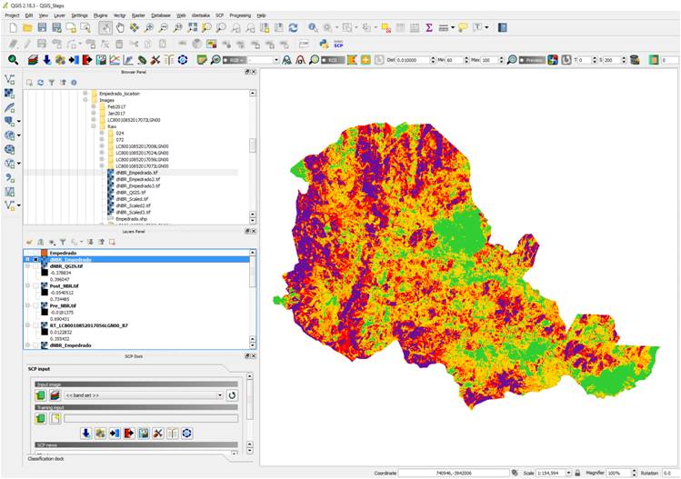
Figure 22. Screenshot of QGIS window after classifying the Burn Severity according to USGS standard.
7. Area Calculation
In order to quantify the area in each burn severity class, the statistics of the raster must be calculated. A transformation of the raster, so that all pixels are assigned one value for each burn severity class is necessary. in addition to this we excluded regrowth in the classification and applied the full USGS table of classification as shown here.
First, open the raster calculater to multiply all values by 1000. Select the dNBR layer, here named USGS_Fire, so that it shows up in the Expression field and multiply it by 1000. The click on Reference layer and select the same layer (Skip this step if you're using a QGIS 2.18.21). Lastly, set the output file name and directory. All other fields can be left as default.
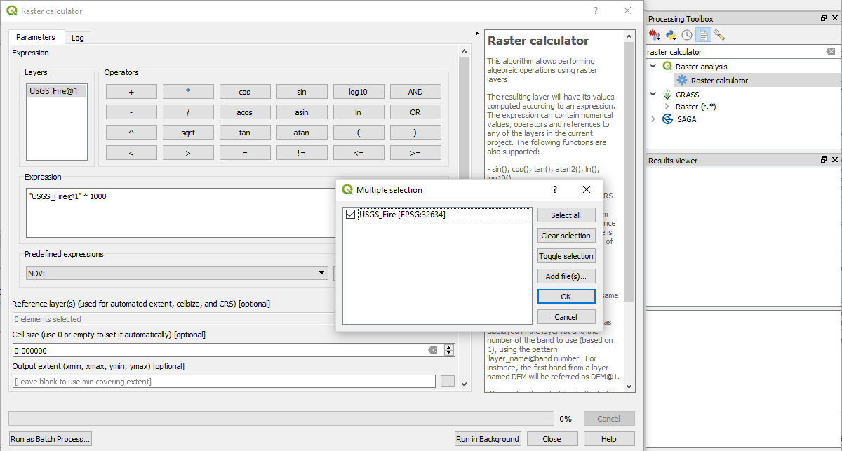
Figure 23. Appyling raster calculator to get integer values.
Second, attribute a class for each of the values just as in the previous style section. This time the underlying information is overwritten so that statistics can be calculated for each class. Open a blank note pad document and enter the following:
-1000 thru -251 = -2 # Enhanced Regrowth, high (post-fire)
- 250 thru -101 = -1 # Enhanced Regrowth, low (post-fire)
- 100 thru 99 = 0 # Unburned
100 thru 269 = 1 # Low Severity
270 thru 439 = 2 # Moderate-low Severity
440 thru 659 = 3 # Moderate-high Severity
660 thru 1300 = 4 # High Severity
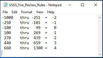
Figure 24. Rules for which pixels are attributed to which class.
Make sure that the Enhanced Regrowth, high (-2) class and High Severity class (4) are extended to fully cover the values of the scene studied.
Then, search for r.reclass in the Processing Toolbox. Select the raster layer that was created in Step 1 and load the Notepad .txt file. Save the output as Reclassified. Leave all other values as default.
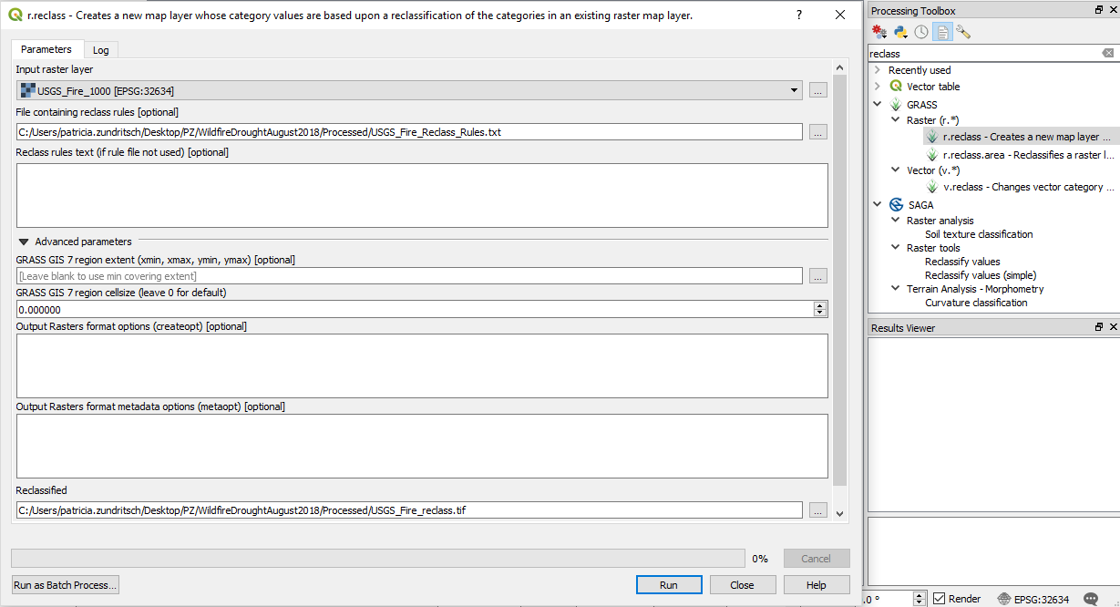
Figure 25. Screenshot of QGIS r.reclass function to attribute a class to groups of values.
Finally open use the Processing Toolbox search bar to find r.report. In the field Raster layer(s) to report on navigate to the reclassified raster layer. Then select the units of choice. In this case we chose h [hectars] and save the Reclass_report_hectars.txt file.
Units to report
Options: mi, me, k, a, h, c, p
mi: area in square miles
me: area in square meters
k: area in square kilometers
a: area in acres
h: area in hectares
c: number of cells
p: percent cover
The result can be seen in figure 27 below and can be copied into excel for further use or presentation.
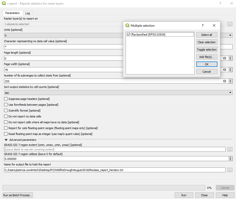
Figure 26. Calculation of raster statistics with r.report.
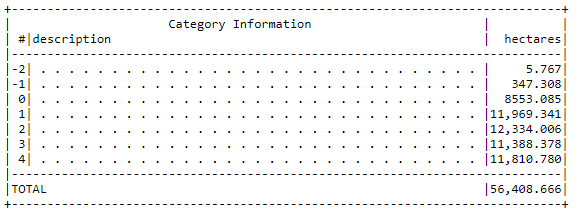
Figure 27. Notepad report of raster statistics.
ADDITIONAL STEPS: Composing the map
This section will demonstrate how to prepare the map to be delivered, i.e. including legend, scale and title. To facilitate the understanding, this section is explained in bullet points.
- In the menu toolbar, go to Project -> New Print Composer and assign a name to your project. This will open a white canvas.
- In the Print Composer window, go to Layout -> Add map. Once the Add Map button is active, hold the left mouse button and drag a rectangle where you want to insert the map (Figure 27).

Figure 27. How to add a map in Print Composer.
- Go to Layout -> Move Content to move the map inside the canvas.
- To insert the legend, go to Layout -> Add Legend and select where you would like the legend to be, holding the left button on the mouse. You will see that it adds all the layers that were in QGIS main window. To have only the relevant layers in the legend, we will delete the unnecessary ones.
- To delete the unnecessary items in the legend, on the right-hand side of the screen, go to Item properties tab. You will see all the items in you legend under Legend items. Deselect Auto update to start removing. Select all layers except the classified raster and click the minus button on the bottom to remove them (Figure 28).

Figure 28. Deleting unnecessary items from the legend.
- Also remove the unnecessary items under the classified map, as shown in Figure 25.

Figure 25. Removing items from the legend of the classified map.
- Add the scale by going to Layout -> Add Scalebar and click where in the canvas you would like to add it. You can change how many segments and units you would like to have on the scale by changing the Scalebar properties on the right-hand side of the window.
- Add the title by going to Layout -> Add Label and click where in the canvas you would like to add it. You can change the text, font and size by changing the Label properties on the right-hand side of the window.
- Add the North arrow by going to Layout -> Add Image and click where in the canvas you would like to add it. You can select the image you would like by going to Search directories and selecting one on the right-hand side of the window.
- If you would like, you can also add more items to your map under Layout in the menu toolbar, such as shapes.
- You can also export it as an image or a PDF. For that, go to Composer in the menu toolbar and choose the suitable option: Export as Image, Export as PDF or Export as SVG.
Figure 26 is an example of a final map for Burn Severity in Empedrado, Chile.

Figure 26. Final Burn Severity map for Empedrado, Chile, using QGIS.