The aim of this step-by-step procedure is the generation of a burn severity map for the assessment of the areas affected by wildfires. The Normalized Burn Ratio (NBR) is used, as it was designed to highlight burned areas and estimate burn severity. It uses near-infrared (NIR) and shortwave-infrared (SWIR) wavelengths. Healthy vegetation before the fire has very high near-infrared reflectance and low reflectance in the shortwave infrared part of the spectrum, in contrast to recently burned areas that have a low reflectance in the near-infrared and high reflectance in the shortwave infrared band. More information about the NBR can be found here. The NBR is calculated for images before the fire (pre-fire NBR) and for images after the fire (post-fire NBR) and the post-fire image is subtracted from the pre-fire image to create the differenced (or delta) NBR (dNBR) image. dNBR can be used for burn severity assessment, as areas with higher dNBR values indicate more severe damage whereas areas with negative dNBR values might show increased vegetation productivity. dNBR can be classified according to burn severity ranges proposed by the United States Geological Survey (USGS).
Data required for this practice:
- Sentinel 2 pre-fire NIR and SWIR images
- Sentinel 2 post-fire NIR and SWIR images
- Shapefile of Empedrado area, Chile
- QGIS software
Download the data
Download the shapefile
The study area that was used for the recommended practice is Empedrado Commune, located in the Province of Talca, Maule region, Chile. The shapefile was obtained through the Universidad de La Frontera, Temuco, Chile (Albers, C., 2012. Coberturas SIG para la enseñanza de la Geografía en Chile).
To download the shapefile, please click here.
Download the images
1. Open the Copernicus Data Space Ecosystem
For this procedure, the Copernicus Data Space Ecosystem website was used to download the images.
2. Register as a User
First, you should have an account in order to be able to access the data. On the upper right corner, click on the 'Login' icon to login or sign up as indicated in Figure 1 by following the 'Sign up' link and following the instructions.

Figure 1a. Registering as a user

Figure 1b. Registering as a user
3. Activate your account
You will receive an email with instructions on how to activate your account.
4. Login to the website
Please go back to the Copernicus website to sign in as a user by clicking on the 'Login' Icon and insert the username and password in the relevant fields. Access the Copernicus Browser, as indicated in figure 2.

Figure 2a. Access to Copernicus Data Space Ecosystem Browser

Figure 2b. Graphical User Interface of Copernicus Data Space Ecosystem Browser
5. Search Criteria
First find the area of interest on the map, which is this case is Empedrado, Chile and draw a rectangle over that region or draw a polygon, using the tool on the top left.

Figure 3. Define a rectangle area of interest
Go to the Search tool and:
- Set the dates for the sensing period (in this case from 1st December 2016 (2016/12/01) to 28th February 2017 (2017/02/28)).
- Select Sentinel-2 as data source.
- Optional: Fill in the Relative Orbit Number (in this case 96).
- Click the search button.

Figure 4. Entering the search criteria
6. Select and download the product
The search will return products containing the area of interest. For this practice images from the dates 20th December 2016 (pre-fire) and 18th February 2017 (post-fire) is used with the following names respectively:
S2A_MSIL1C_20161220T143742_N0204_R096_T18HYF_20161220T145131
S2A_MSIL1C_20170218T143751_N0204_R096_T18HYF_20170218T145150
To download the products click on the download icon.

Figure 5. Download products
Content
QGIS Basics
Data Preparation/Pre-Processing
Step 2: Top of the Atmosphere (TOA) corrections
Processing Steps
Step 3: Calculating the Normalized Burn Ratio (NBR)
Step 4: Calculating delta NBR (dNBR)
Step 5: Applying the cloud mask
Step 7: Setting the ranges according to USGS standard
Additional: Composition of the map
QGIS basics
QGIS is an Open Source Geographic Information System (GIS) licensed under the GNU General Public License. QGIS is an official project of the Open Source Geospatial Foundation (OSGeo). It runs on Linux, Unix, Mac OSX, Windows and Android and supports numerous vector, raster, and database formats and functionalities (QGIS).
To start working, open the QGIS Desktop. Figure 1 illustrates an example of the QGIS Desktop interface, the Browser and Layers Panels and the Map Canvas. The QGIS Browser is a panel from which you can access your database. In the Layers Panel, there is a list of all the layers that you have added to your map. You can also expand collapsed items (by clicking the arrow or plus symbol beside them). This will provide you with more information on the layer’s current appearance.
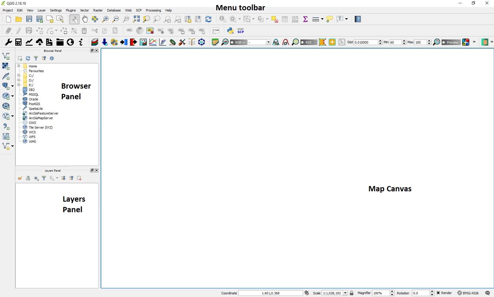
Figure 6. QGIS interface
Burn Severity
The images and the shapefile of the study area should have already been downloaded in order to start processing.
- The folder containing the pre-fire images (for this procedure, the Sentinel-2 images name used for pre-fire is T18HYF_20161220T143742)
- The folder containing the post-fire images (for this procedure, the Sentinel-2 images name used for post-fire is T18HYF_20170218T143751)
- The shapefile of the assessed area
1. Open images in QGIS
There are two ways you can open the downloaded images in QGIS. One way is using the browser panel (explained in section a), and the other way would be using menu toolbar (explained in section b). You can choose which way is more suitable for you.
The layers that will be added were acquired by Sentinel-2 before and after the fire. The bands that will be used to calculate the Normalized Burn Ratio (NBR) are the Near Infrared (NIR) and Shortwave Infrared (SWIR), which correspond to band 8A and band 12, respectively.
a. Opening images using the browser panel
Please find where you have stored your images (Get in the product folder -> GRANULE -> L1C... -> IMG_DATA), select the bands that are going to be used for NBR. Once each layer has been selected, double-click it to add it to the Map Canvas or you can also drag-and-drop the layer to the Map Canvas (Figure 7).
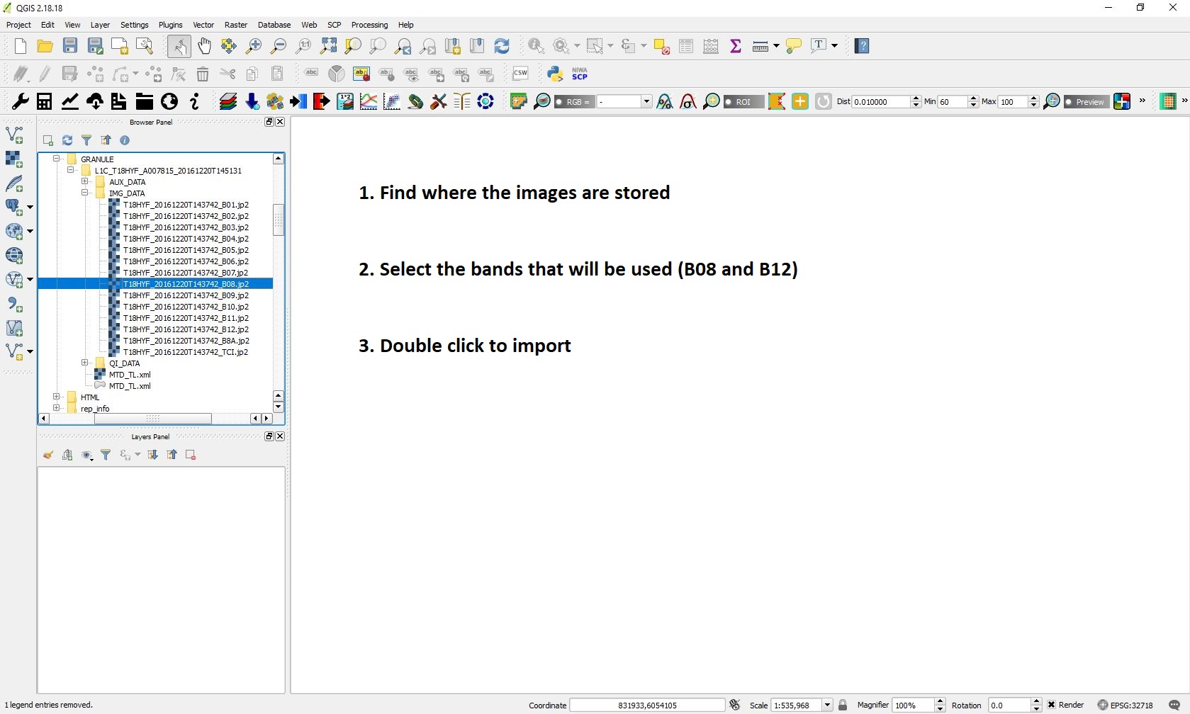
Figure 7. Opening images using the browser panel in QGIS
b. Opening images using the menu toolbar
To open the images using the menu toolbar, please click on Layer -> Add Layer -> Add Raster Layer (Figure 8). This should open a window where you can find the folder where the bands are stored (Get in the product folder -> GRANULE -> L1C... -> IMG_DATA). When you find them, select and click open for each of the bands.
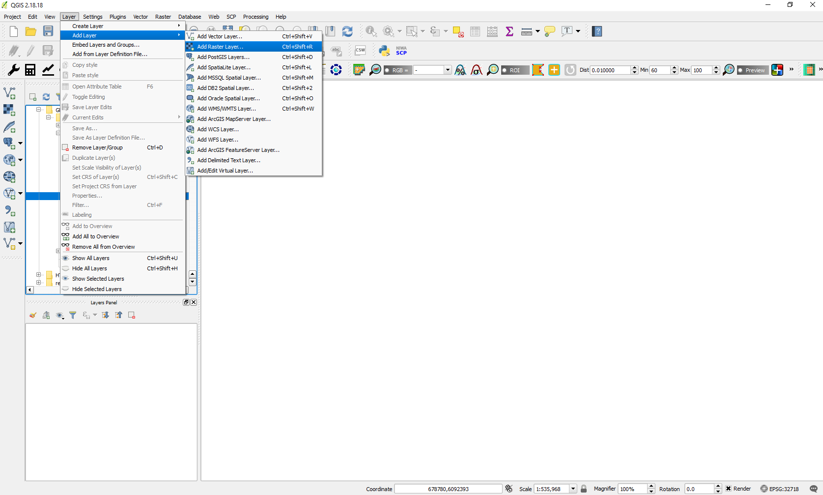
Figure 8. Opening images using the menu toolbar in QGIS
After the images are loaded into Map Canvas, you should see them on the layers panel, as indicated by the red box in Figure 9.
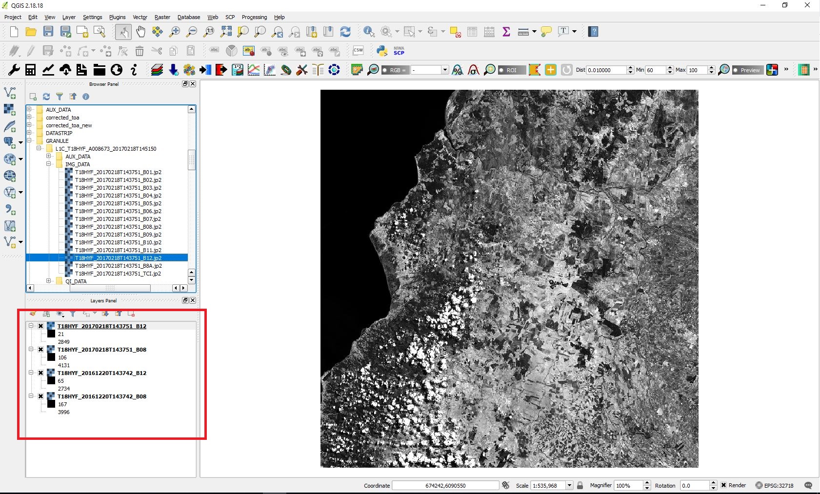
Figure 9. Screenshot demonstrating how the Layers Panel should look after loading the relevant bands.
2. Top of the Atmosphere (TOA) corrections
The first step before start calculating the NBR is to apply a top of the atmosphere correction. This is done in order to separate the actual reflectance that was emitted from the objects on the Earth's surface (which is what we need) from the atmospheric disturbances that are part of the reflected energy recorded by the sensor. For more information about the correction here.
2.1. Installing the Semi-Automatic Classification Plugin
Firstly, please be sure that you have administrator rights on your computer, i.e. that you are authorized to install software and plugins. For this procedure, you will be required to install a plugin.
To correct for the TOA in QGIS, the Semi-Automatic Classification plugin is used. So before correcting, please be sure that you have the plugin installed. To install it, please go to Plugins -> Manage and install plugins… (Figure 10).

Figure 10. How to install plugin (red box)
After clicking on Manage and Install Plugins… a new window should open where you can search for plugins to be installed. Please type on the search box 'Semi-Automatic'; after typing it should automatically show you the plugins options that correspond to the search (Figure 11). After selecting the Semi-Automatic Classification (SCP) Plugin, please click install on the bottom right corner of the window (indicated by the red box in Figure 11).
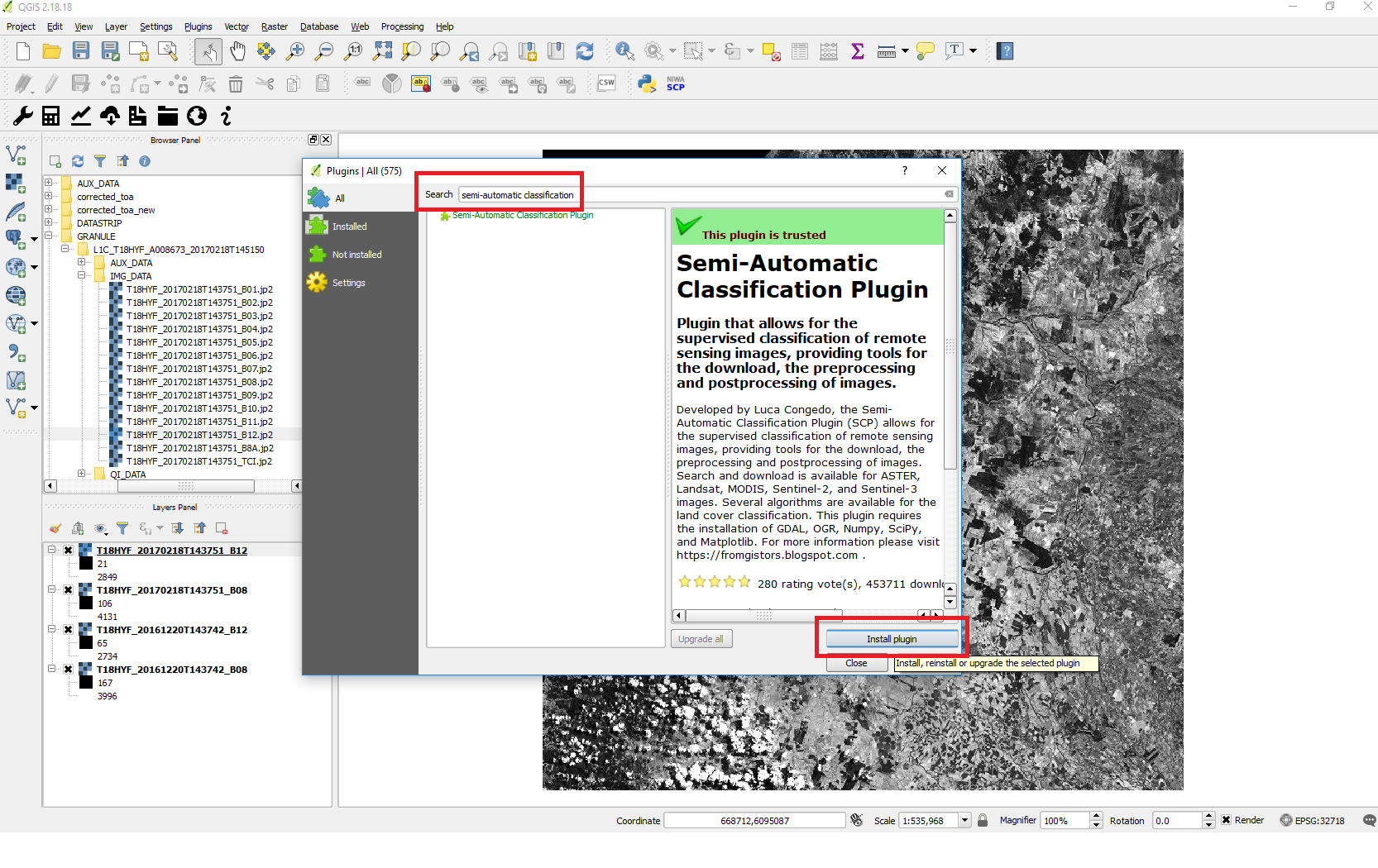
Figure 11. Plugins' search in QGIS.
2.2. Open the SCP pre-processing Window
So now there should be an SCP icon on your menu toolbar. Please go to SCP -> Preprocessing -> Sentinel-2, as demonstrated in the red box in Figure 12.

Figure 12. Path to follow to SCP -> Preprocessing -> Sentinel-2 (red box).
After following the path and clicking Sentinel-2, a new window should open, such as the one shown in Figure 13. Click first on the yellow icon indicated by a red box in Figure 13 to select the folder where your images are and then on the icon below to select the folder where metadata is (file MTD_MSIL1C).
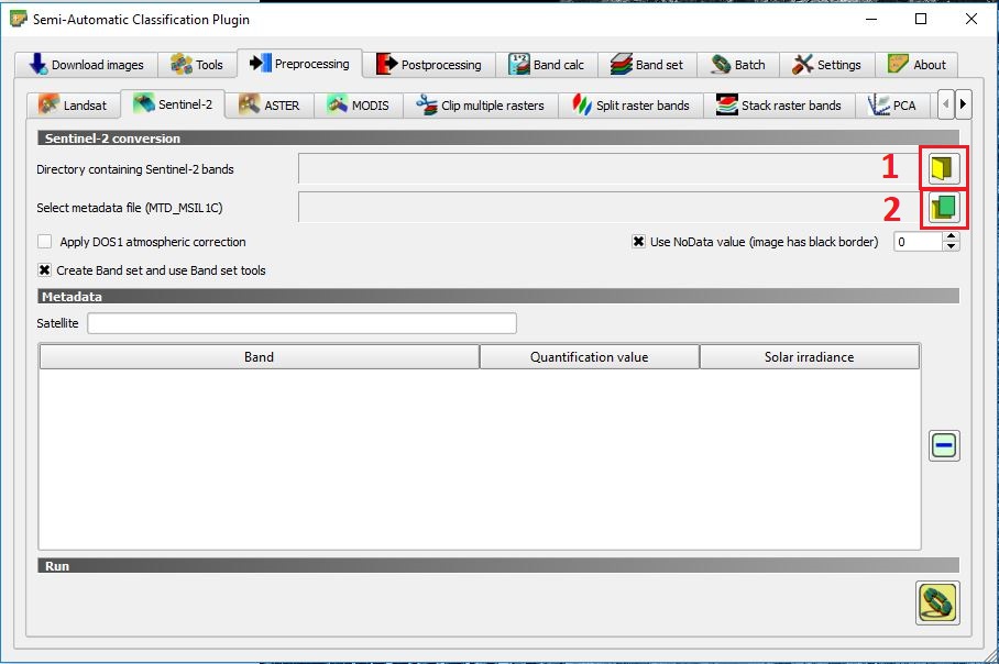
Figure 13. Semi-Automatic Classification Plugin Preprocessing window.
2.3. Select the folder that contains the pre-fire images
After selecting the folder that contains the pre-fire images, you should see your folder path on the 'Directory containing Sentinel-2 bands' and on the 'Select metadata file (MTD_MSIL1C)' (Figure 14). Below that you should also see the bands that are in the selected folder (Figure 14).
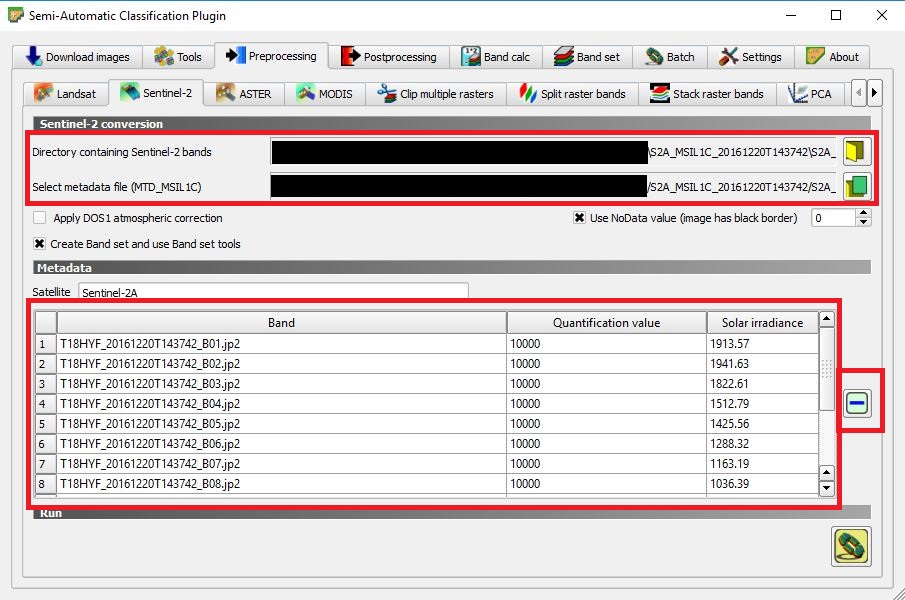
Figure 14. SCP window after selecting the folder with Sentinel-2 pre-fire images and the metadata file
2.4. Top of the Atmosphere (TOA) corrections
On the SCP processing window, please select Apply DOS1 atmospheric correction. Leave also Use NoData value (image has a black border) option selected. Select the bands that will not be used during the NBR process and remove them (click the 'minus' icon in the red box indicated in Figure 14 on the right-hand side), i.e. remove all bands except 8A and 12. Your SCP window should look similar to the one in Figure 15. Finally, click run (icon in a red box at the bottom of Figure 15)
TIP: You can select multiple files to be removed by holding the Ctrl key on your keyboard while selecting the files.

Figure 15. SCP window showing the bands to be corrected
Please note that after clicking run, it will ask you to select the folder where the corrected images will be stored. In case you do not already have a folder created, simply click on create a folder to create a new one (Figure 16).
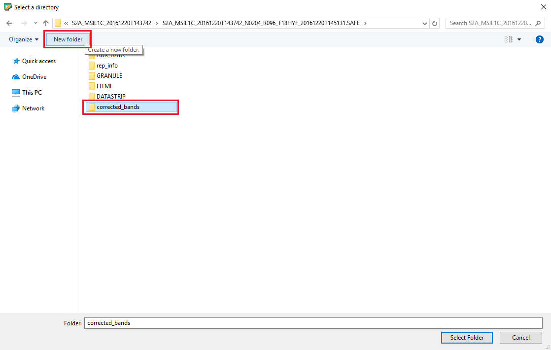
Figure 16. Screenshot showing the icon to create a new folder to store the corrected images.
This process could take a few minutes depending on the computer’s configuration. The progress can be monitored in the main window of QGIS, where a progress bar is shown.
Please note that the corrected bands are automatically added to the layers panel, with 'RT' in front of the file name.
Now, the pre-fire images have already been corrected, however, the post-fire images still need to be processed for the TOA corrections. Please also correct the post-fire images following the same steps as the ones gone through for the pre-fire images, i.e. from step 2.3. Be sure to use to the correct folder containing the bands of post-fire and the metadata file.
After having the pre- and post-fire images corrected, your QGIS should be looking similar to the one shown in Figure 17.

Figure 17. Screenshot of the processing done until now.
2.5 Cloud Mask
The following steps are important in the case that there are clouds in the image. Sentinel-2 level 1C product contains a cloud mask that masks the majority of clouds but it is not very accurate. For this reason, even though we will use this mask, it might not include all the clouds in the image.
You can find the cloud mask in the product folder -> GRANULE -> L1C... -> QI_DATA -> MSK_CLOUDS_B00.gml. First, please load the cloud mask for the pre-fire image either by using the browser panel (find the file and double-click to add it) or the menu toolbar (Layer -> Add Layer -> Add Vector Layer) as it was also described in the first step of the Image Processing section.
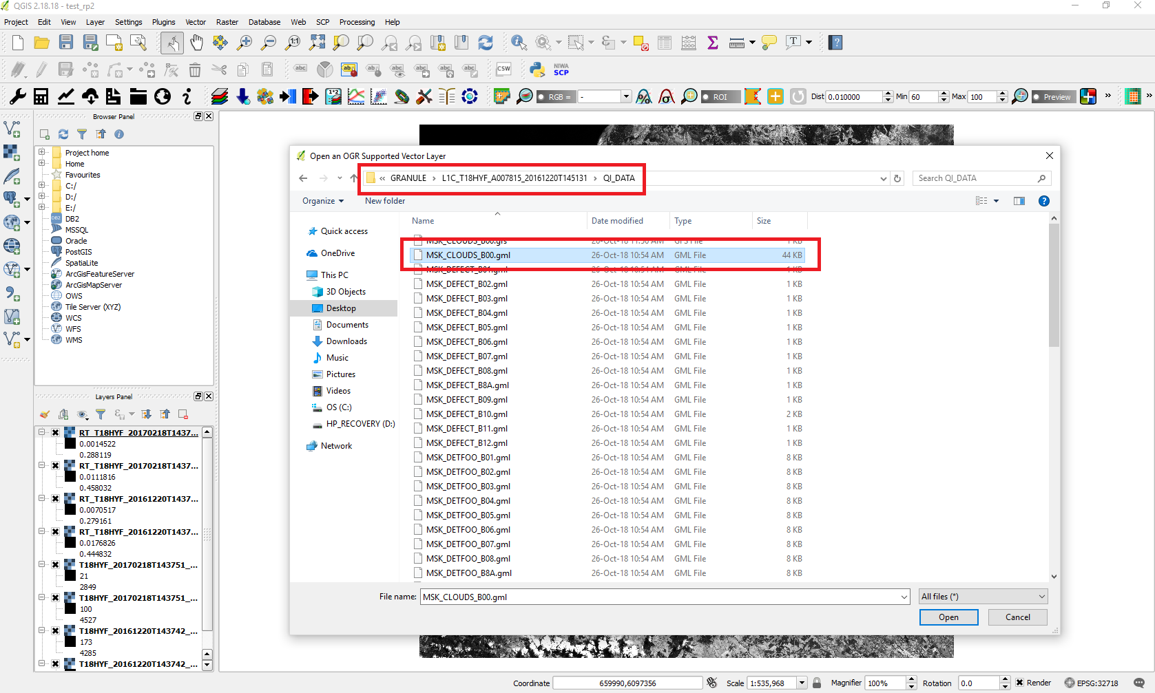
Figure 18. Open the cloud mask file
After you load the file, it will appear in the layers panel. Then right click on the name and select Save as... to save it as a shapefile.
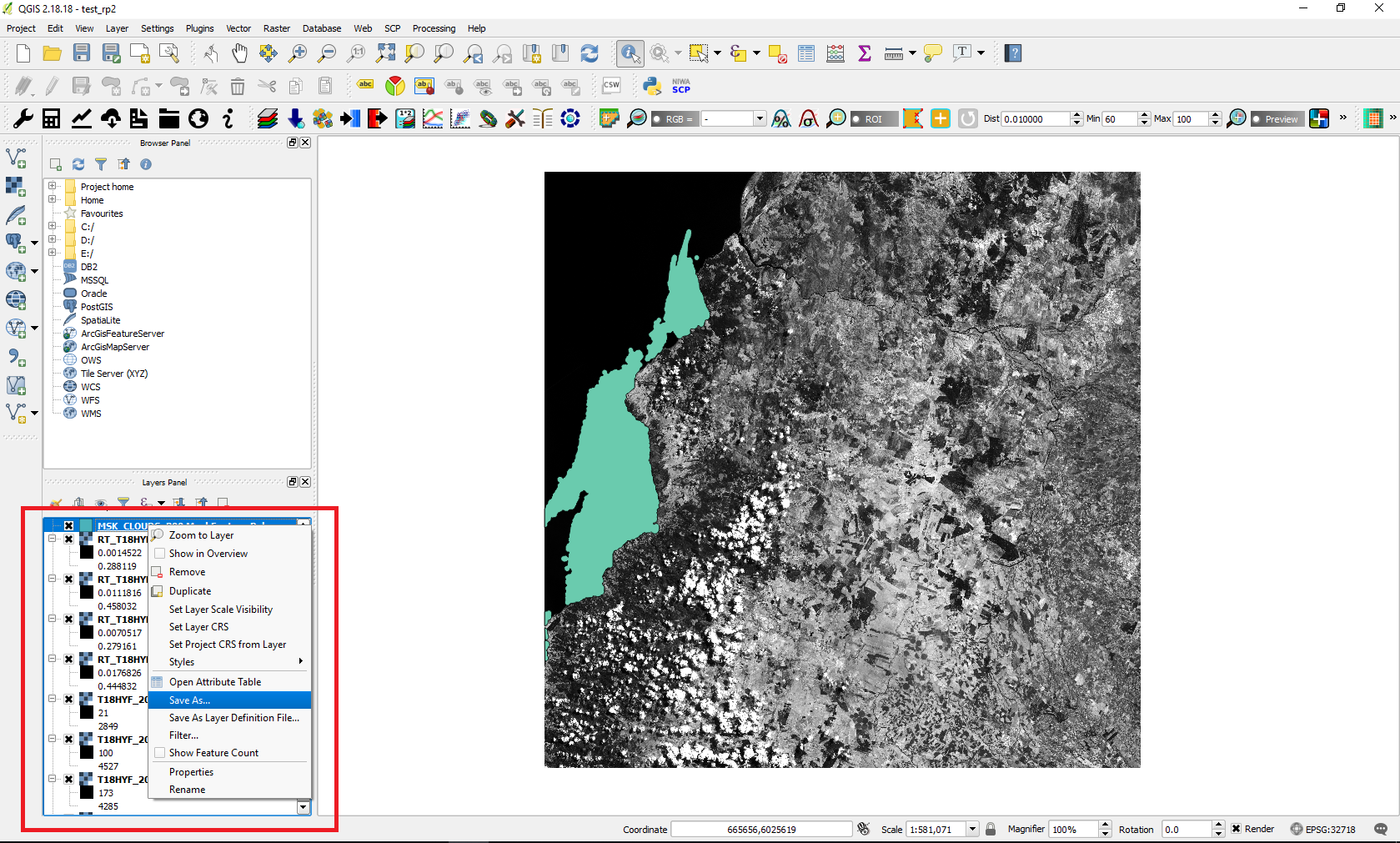
Figure 19. Save as shapefile.
Specify the file name (in this case clouds_december) and the directory and set the Coordinate Reference System (CRS) to match the (CRS) of the rest files.

Figure 20. Set the Coordinate Reference System
After the creation of the new shapefile, right click on it and select Open Attribute Table. Enable the Toggle editing mode by clicking on the first icon and then open the field calculator (red boxes in Figure 21).
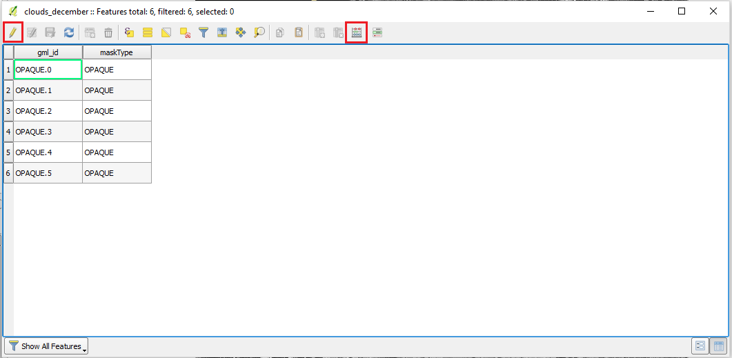
Figure 21. Attribute table
Then fill in the name of the new field (in this case value) at the 'Output field name' and edit the expression at the bottom by writing 1 (Figure 22). In this way, a new field will be created with the field name 'value' and all the features will have the value 1. This is performed in order to be able to use this value later in the processing. Then save the changes (third icon) and disable Toggle editing mode.
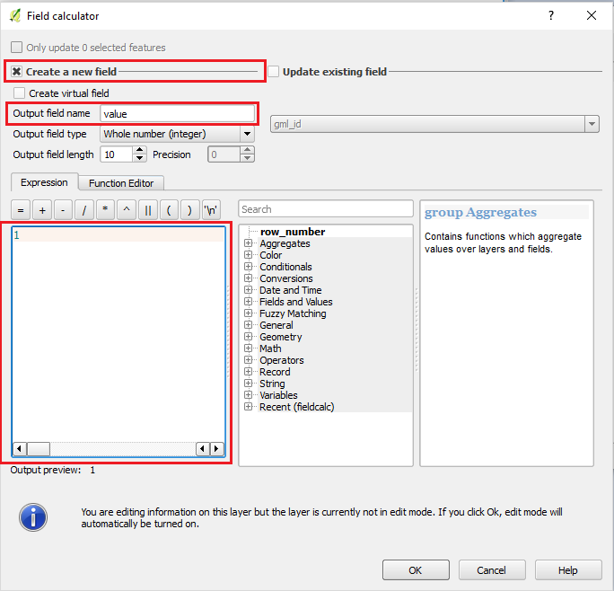
Figure 22. Field calculator
Then follow the same procedure for the cloud mask of the post-fire image.
IN THE FOLLOWING STEPS, ONLY THE CORRECTED IMAGES WILL BE USED.
3. Calculating the Normalized Burn Ratio (NBR)
NBR is calculated using the NIR and SWIR bands of Sentinel-2 in this practice using the formula shown below:
NBR = (NIR - SWIR) / (NIR + SWIR)
NBR = (B8A - B12) / (B8A + B12)
In order to calculate NBR in QGIS, the tool Band Calc will be used. So please go to SCP -> Band Calc. After selecting the Band Calc tool, it should open a new window, as indicated by the red box in Figure 23.

Figure 23. The Band Calc tool.
To assess burn severity, NBR should be calculated for both pre and post-fire images. This will then enable the calculation of their difference (dNBR) and burn severity.
3.1 Calculate pre-fire NBR
In the case that the band list is empty you should press the refresh list button ( ) on right side in order to update the list of the raster files available for calculation. Then, you should enter the expression to calculate NBR for the pre-fire images. To add the files that will be used in the expression, you can simply double click on their names and it will add them to the expression. In this case, the following expression was used.
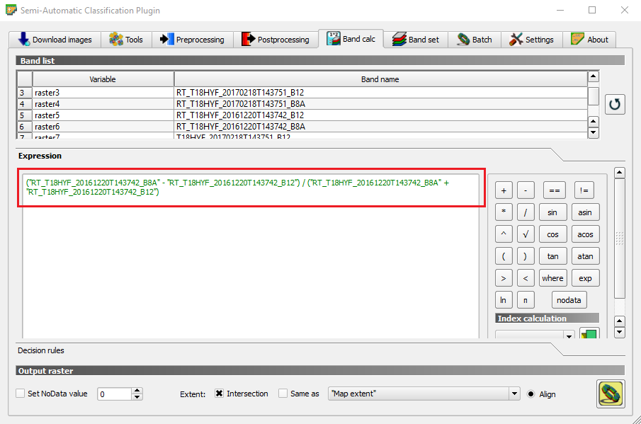
Figure 24. Screenshot of the expression for the NBR calculation.
After inserting the expression, click Run (icon in the bottom right corner, indicated in Figure 24). After clicking Run, you will be able to select which folder you would like to save the new file and you can name the file as you prefer. During this procedure, it was named as Pre_NBR.
3.2 Calculate post-fire NBR
After the pre-fire NBR calculation enters the expression to calculate NBR for the post-fire images following the same procedure as before. During this procedure, the file was named as Post_NBR.
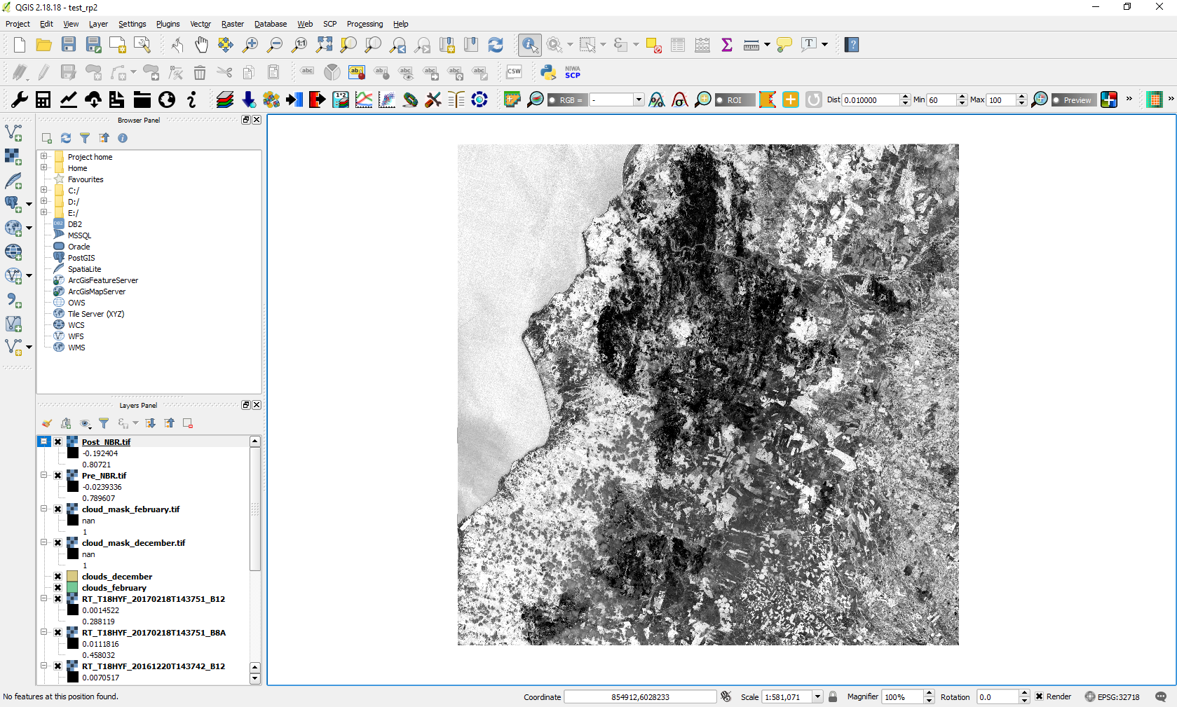
Figure 25. Screenshot of the processing done after running the pre- and post-fire NBR.
4. Calculating delta NBR (dNBR)
After calculating NBR for both pre and post-fire images, it is possible to determine their difference and obtain dNBR. Therefore, first, you should calculate the difference between the NBR before and after the fire, referred to as dNBR during this practice. For that, the NBR of the post-images is subtracted from the NBR of the pre-images, as shown in the formula below:
dNBR = pre-fire NBR – post-fire NBR
Open the Band Calc tool again (SCP -> Band Calc) and click the refresh list icon again, so the new calculated files will also appear. Remove the previous expression and insert the following one:
After clicking Run, please select the folder where you would like the new file to be added into and the name of the file. The calculated dNBR should be added automatically to the Layers Panel and Map Canvas. By now, you should be seeing a similar screen like the one shown in Figure 26.
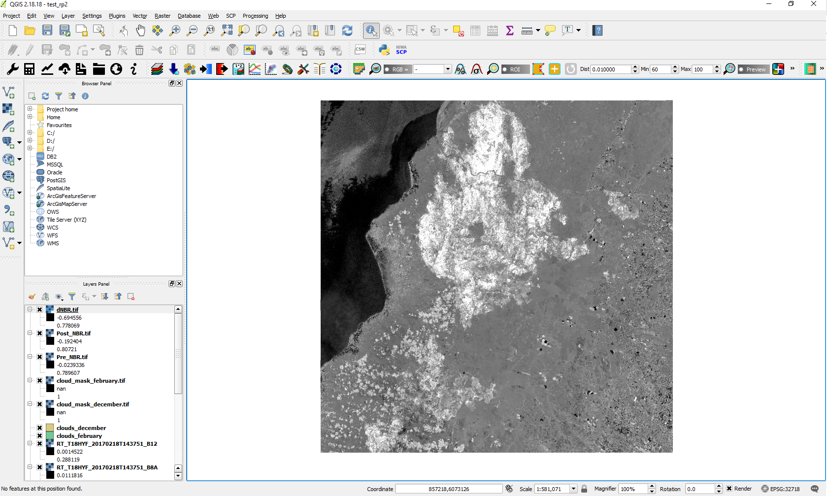
Figure 26. Screenshot of the processing done after running dNBR.
5. Applying the cloud mask
After the calculation of the dNBR, we will mask out the cloud areas. So, please go through the menu toolbar Raster -> Conversion -> Rasterize. Specify the input shapefile (clouds_december in this case) and the output file (dNBR tif file that was created in the previous step). The result will be overwritten on the dNBR raster file. Afterwards, click on the pencil icon at the bottom (red box in Figure 27) and fill in '-burn 500'. This option is used in order to give the value 500 for the pixels masked as clouds. You can use any other value, that is larger or smaller from the values already existing so that it can be easily distinguished.
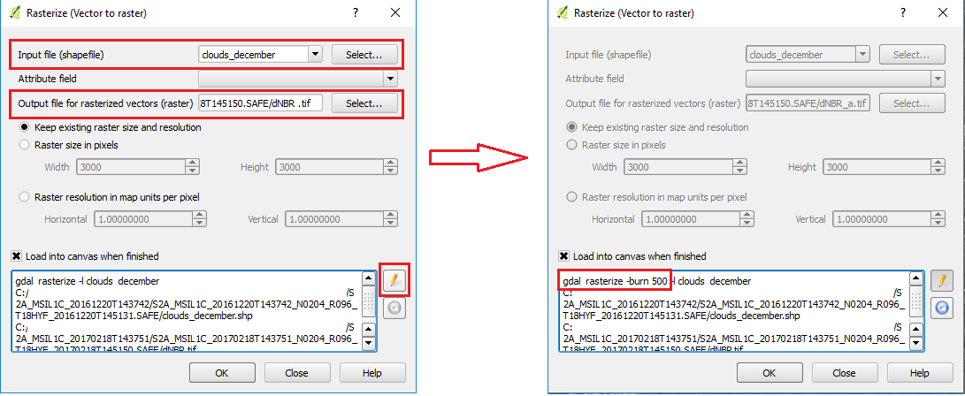
Figure 27. Rasterize
After this command is finished do the same with the other shapefile for the clouds of the post-fire image, using as output the file that was created from the last step (i.e. the raster file containing dNBR and pre-fire cloud mask).
The result is then loaded on the canvas. Depending on the value you gave to clouds the image can look as black and white. In order to see the dNBR information, right click on the layer name and select Properties. Then the 'Layer Properties' dialogue should open in a new window and please select the tab called Style and change the max value to e.g. 1 (Figure 28).
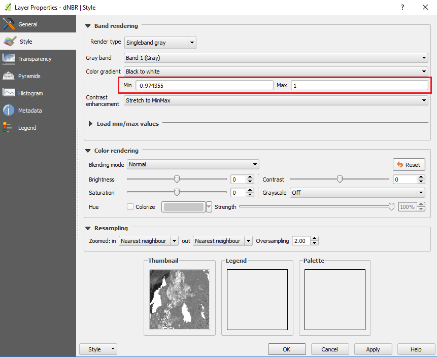
Figure 28. Layer properties
6. Clipping the image
The shapefile of the correspondent area (i.e. Empedrado) will be used to clip the raster dNBR to obtain an image reflecting only the study area. As during this recommended practice, we are using the area of Empedrado region in Chile, the administrative boundary of the aforementioned area will be used.
6.1. Adding the shapefile
In order to add the 'Empedrado' shapefile, you can either use the browser panel (find the shapefile and double-click to add it) or the menu toolbar (Layer -> Add Layer -> Add Vector Layer) as it was also described in the first step of the Image Processing section. After adding the shapefile, you should see the shapefile on top of your images, as it can be seen in Figure 29. Please note that the shapefile colour shown may differ, as it is automatically selected by QGIS.
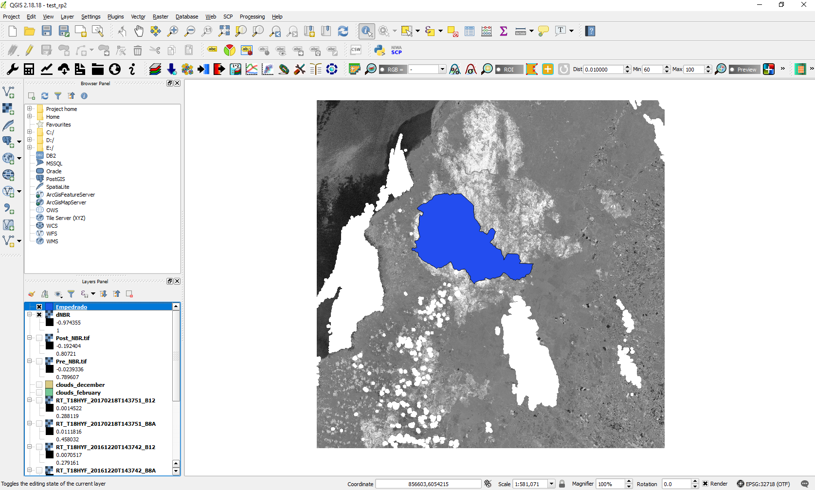
Figure 29. Screenshot of QGIS window demonstrating the Empedrado shapefile in blue.
6.2 Clipping dNBR
In order to crop the image, please go through the menu toolbar and click SCP -> Preprocessing -> Clip multiple rasters and the SCP window will open (Figure 30).
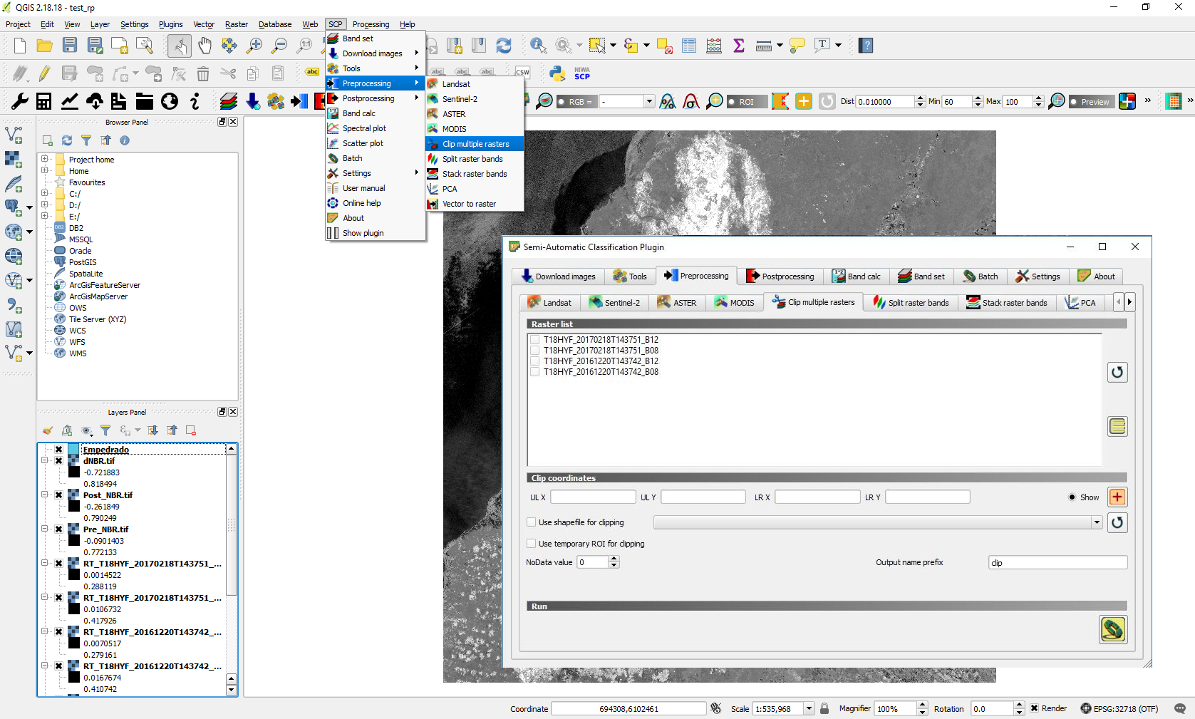
Figure 30. SCP window and Clip multiple rasters tool
Select the dNBR raster, after refreshing the list by clicking the refresh list button () on the right side. Then select the option 'Use shapefile for clipping' and the refresh button in order to show the shapefile Empedrado. Then change the 'Output name prefix' to Empedrado and click run on the bottom. Select a folder where the clipped raster will be saved.
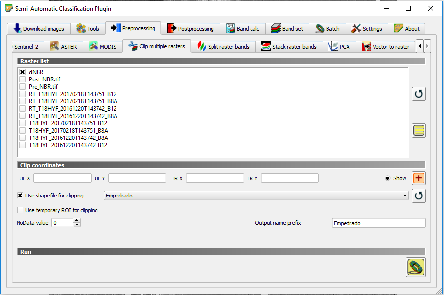
Figure 31. Clip multiple rasters tool and options that should be selected to clip dNBR
After clipping, the raster showing only the Empedrado area is automatically loaded into the Layers Panel and Map Canvas. In order to see only the study area in Map Canvas, deselect the other raster files in the Layers Panel, leaving only the clipped raster selected. After that, you should be seeing the clipped area on your Canvas.
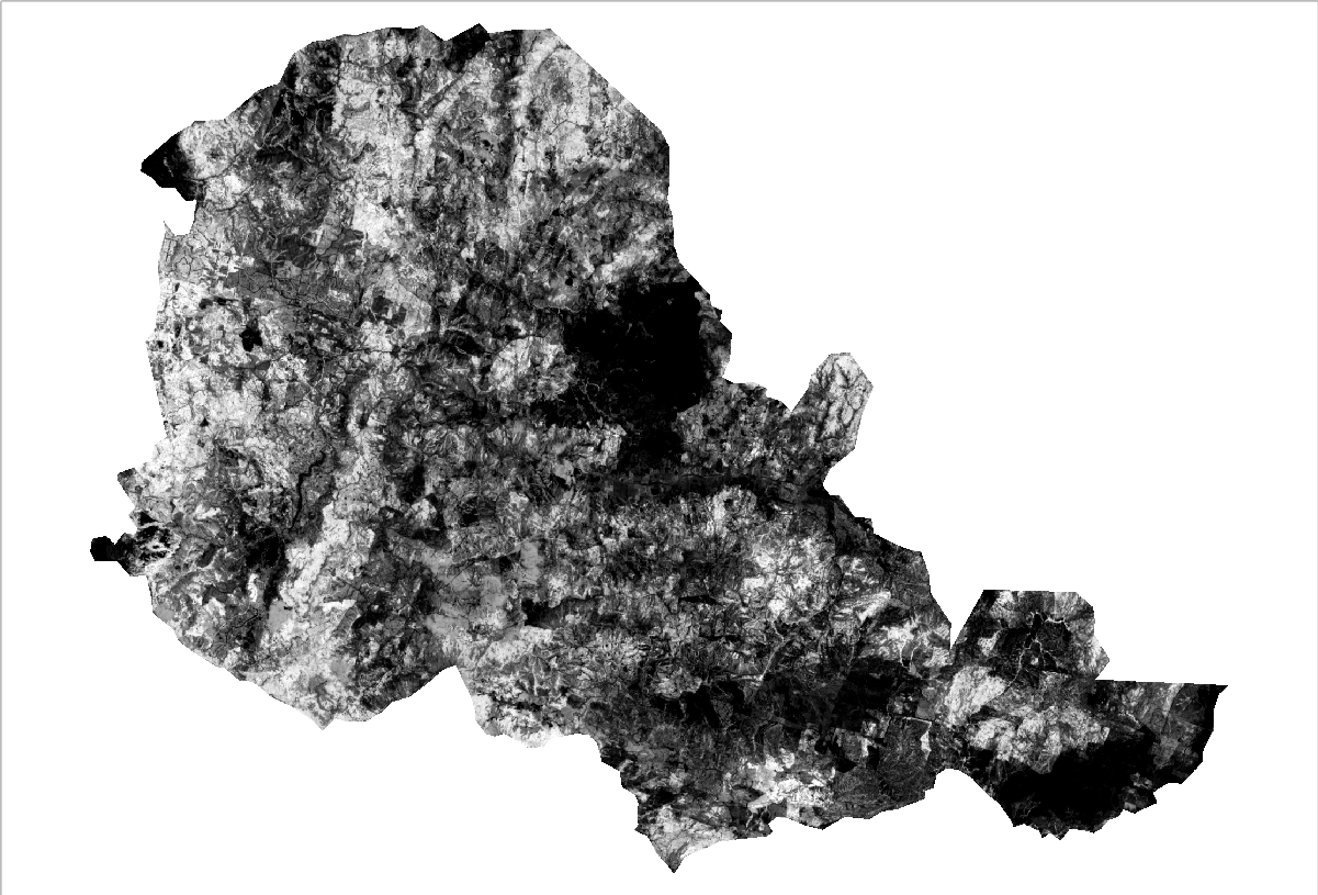
Figure 32. Screenshot of the clipped raster.
7. Setting the ranges according to USGS standard
USGS standard will be used to classify the burn severity map according to the proposed number ranges, as explained here.
7.1. Classifying dNBR
To classify the map, right-click the file name under the Layers Panel and select Properties.
After clicking properties, the 'Layer Properties' dialogue should open in a new window. Please select the tab called Style. In this tab, please change the features as demonstrated below:
- Change the Render type to Singleband Pseudocolor;
- Add 5 classes by clicking the plus icon at the bottom (Figure 33)
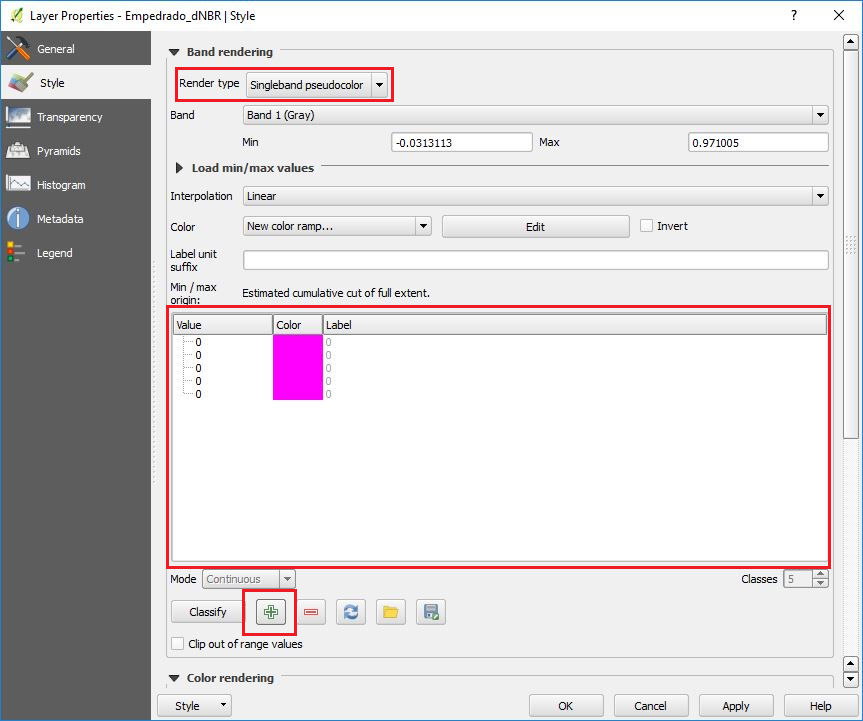
Figure 33. Layer Properties dialogue window.
Now we will change the values (according to USGS standard) and colours of the Layer Properties. Please fill out the ranges to match the Layer Properties dialogue shown in Figure 34, which is based on the table shown here. The choice of colours is not standardized and therefore, it is up to the user to choose the colour palette.
Please note: In this case, we do not show any areas of regrowth.
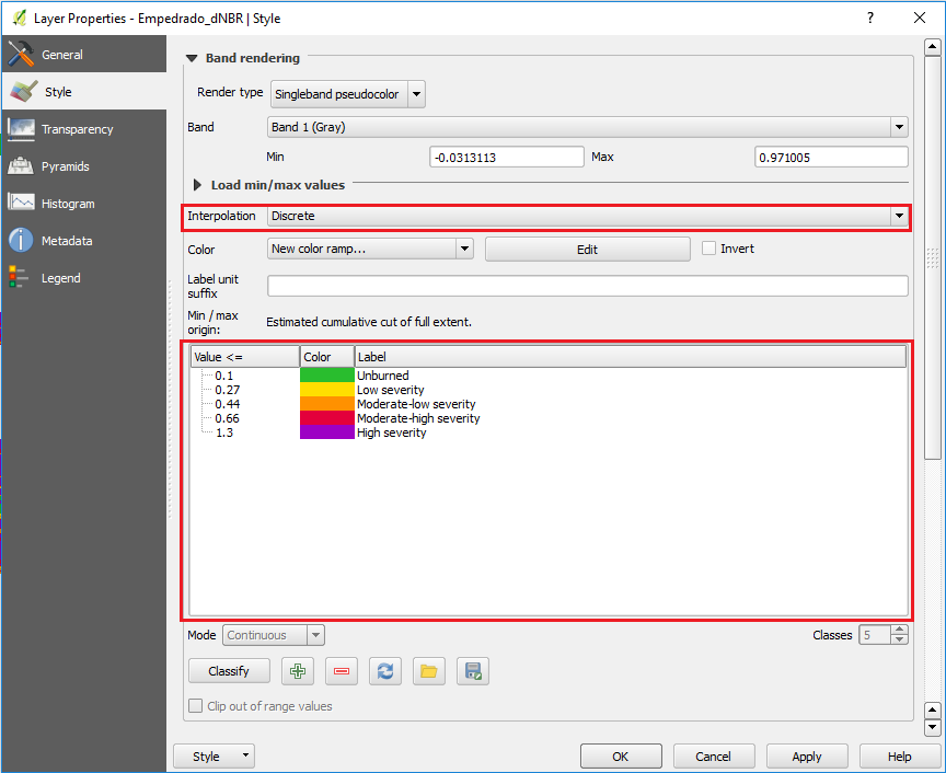
Figure 34. Screenshot of the ranges used for classification.
After inserting the ranges, click Apply and OK. You should then see a similar map to the one in Figure 35.
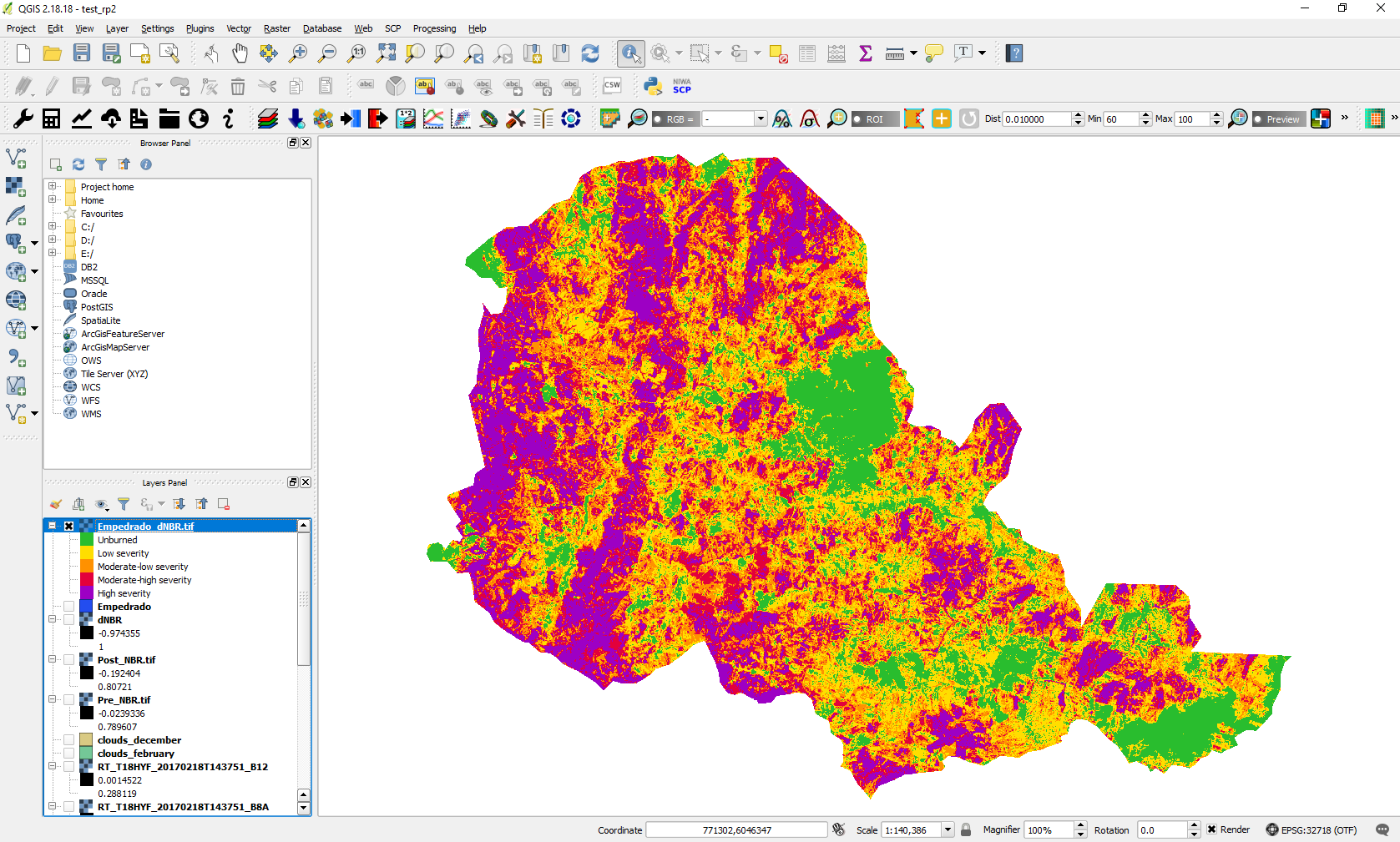
Figure 35. Screenshot of QGIS window after classifying the Burn Severity according to USGS standard.
8. Area Calculation
In order to quantify the area in each burn severity class, the statistics of the raster must be calculated. A transformation of the raster, so that all pixels are assigned one value for each burn severity class is necessary.
First, we will multiply all values by 1000, so please go through the menu toolbar and click Raster -> Raster Calculator. Then specify the 'Output layer' by selecting the output file name and directory. In this case, the name of the file was 'Empedrado_dNBR_1000'. Then, fill in the expression shown in Figure 36 in the 'Raster Calculator Expression' by double-clicking the layer 'Empedrado_dNBR' and typing * 1000.
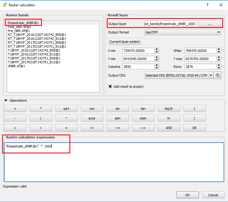
Figure 36. Applying raster calculator to get integer values.
Second, we will attribute a class number to each of the burn severity levels. Thus, in a blank notepad document enter the following and save it as USGS_Fire_Reclass_Rules.txt. Note that the class of clouds (i.e initially value 500 in Empedrado_dNBR raster and value 5*105 for Empedrado_dNBR_1000 is not included in any of the classes.
Now we will reclassify the dNBR raster for Empedrado, based on the classes defined at the previous step. Please go through the menu toolbar and click Processing -> Toolbox and a new panel will open on the right side (Figure 37).
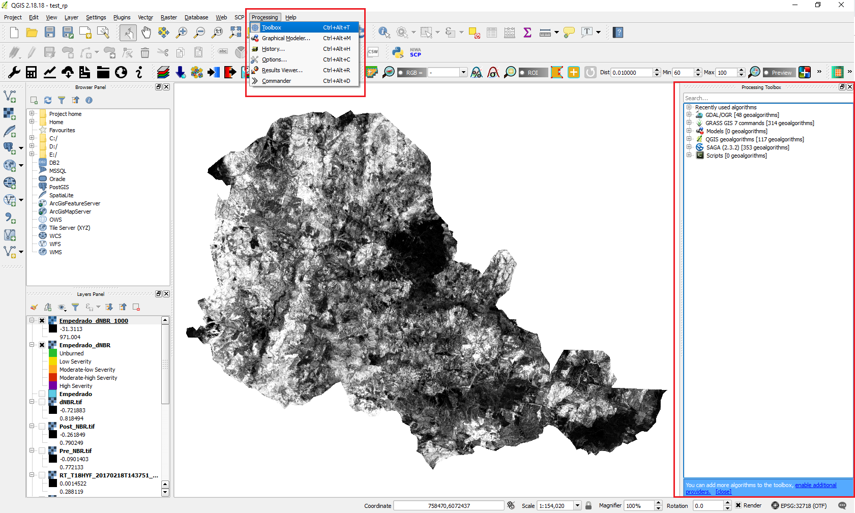
Figure 37. Processing Toolbox
Then, type reclass in the search bar and click on the r.reclass command. A new window will open as it is shown in Figure 38. Specify the 'Input raster layer' (Empedrado_dNBR_1000 in this case) and the text file we created earlier at the 'File containing reclass rules (optional)' (USGS_Fire_Reclass_Rules.txt in this case). Finally, at the 'Reclassified' option, click on them, then select 'Save to file' and specify the directory and file name (Empedrado_dNBR_reclassified.tif in this case). Click on Run at the bottom in order to execute the command. Note that the clouds will be classified as no data because they are not included in any of the defined classes.
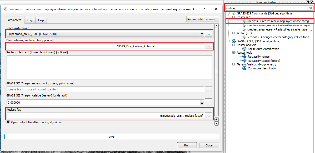
Figure 38. r.reclass command window
Note that after the command is executed, the raster is loaded and it is shown with the name 'reclassified' in the layer panel. You can change the name to Empedrado_dNBR_reclassified by right-clicking on the layer name and select rename.
Now we will calculate the area for each class we defined earlier. So please type report in the search bar of the Processing toolbox and select the r.report command. A new window will open as it is demonstrated in Figure 39. First, you should select the 'Raster layer(s) to report on' by clicking on the and then selecting the raster we created earlier (Empedrado_dNBR_reclassified) (red box in Figure 39). Finally, you should specify the results file under the 'Report' option (Reclass_report_hectar.html in this case).
Note that the units of the calculated area in this practice are in hectares [h]. The other options are:
Options: mi, me, k, a, h, c, p
mi: area in square miles
me: area in square meters
k: area in square kilometres
a: area in acres
h: area in hectares
c: number of cells
p: percent cover
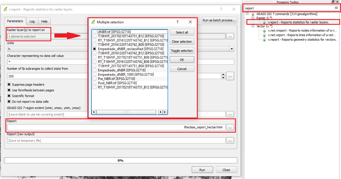
Figure 39. r.report command window
After executing the command (Run at the bottom of the window) a new window will open showing the results.
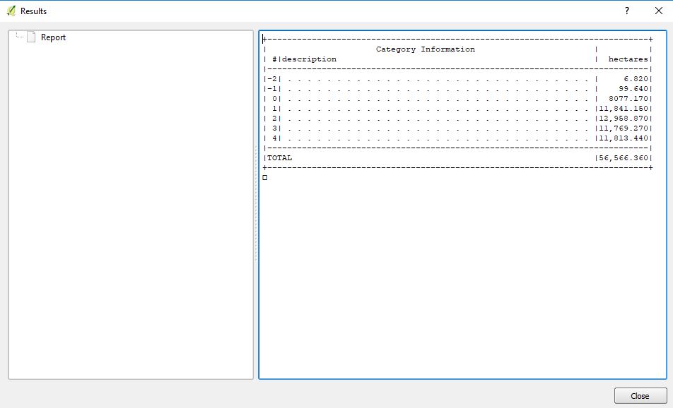
Figure 40. Results of r.report
Note: The area calculation might include information for areas that do not represent vegetation and are misclassified, such as water bodies (e.g. river), settlements, clouds, cloud shadows, roads. Thus, in order to get more reliable results, those areas have to be masked out.
Note: In case you want to check the regrowth of the vegetation after the fire you can use two images after the fire and follow the same procedure as above and include in the classification the classes for enhanced regrowth high and low.
ADDITIONAL STEPS: Composing the map
This section will demonstrate how to prepare the map to be delivered, i.e. including legend, scale and title. To facilitate the understanding, this section is explained in bullet points.
- In the menu toolbar, go to Project -> New Print Composer and assign a name to your project. This will open a white canvas.
- In the Print Composer window, go to Layout -> Add map. Once the Add Map button is active (red box in the left side in Figure 41), hold the left mouse button and drag a rectangle where you want to insert the map (Figure 41).
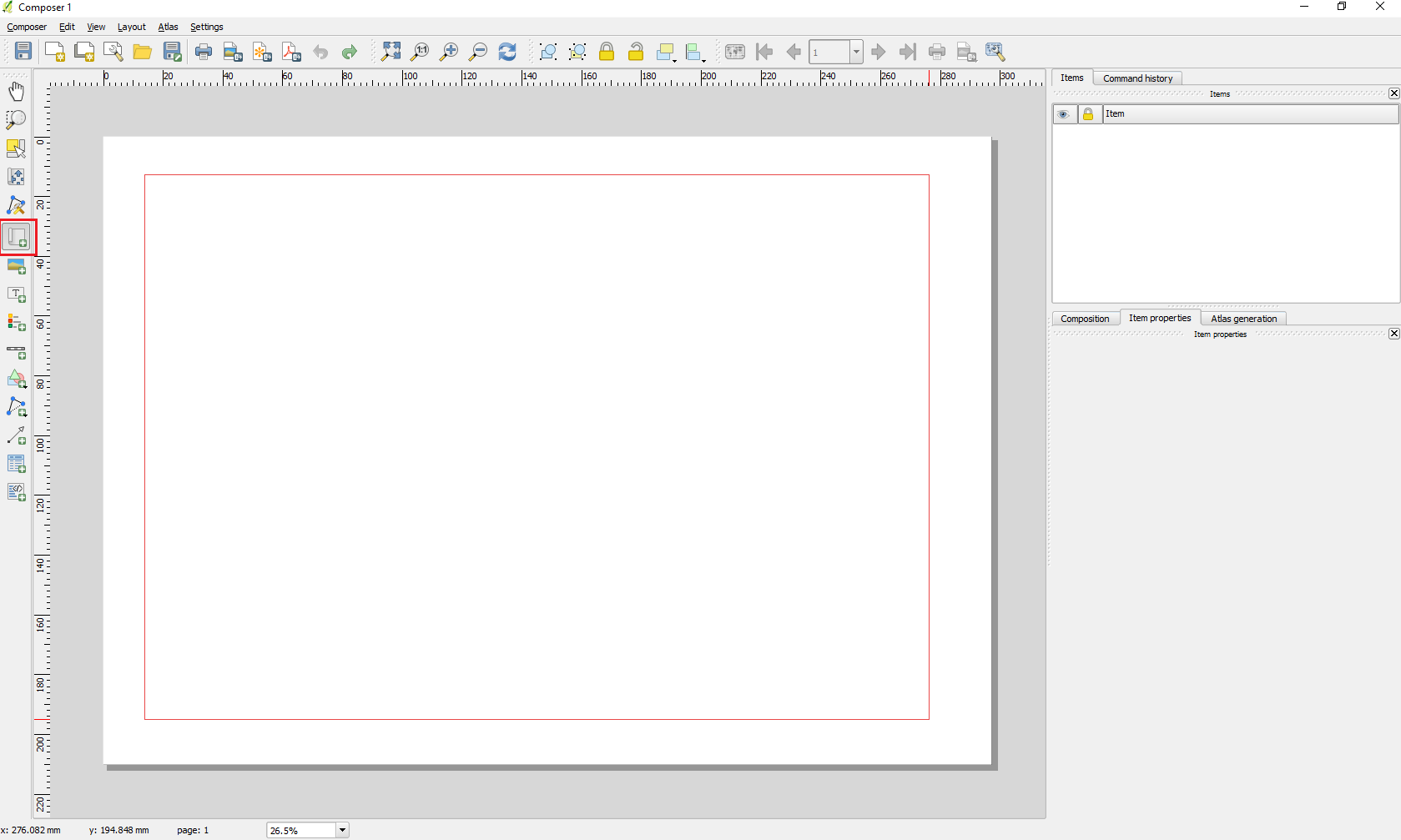
Figure 41. How to add a map in Print Composer
- Go to Layout -> Move Content to move the map inside the canvas. Note that the layer that you want to show in the map should be the only active layer in layer panel in main QGIS window.
- To insert the legend, go to Layout -> Add Legend and select where you would like the legend to be, holding the left button on the mouse. You will see that it adds all the layers that were in QGIS main window. To have only the relevant layers in the legend, we will delete the unnecessary ones.
- To delete the unnecessary items in the legend, on the right-hand side of the screen, go to the Item properties tab. You will see all the items in you legend under Legend items. Deselect Auto update to start removing. Select all layers except the classified raster and click the minus button on the bottom to remove them (Figure 42).

Figure 42. Deleting unnecessary items from the legend
- Add the scale by going to Layout -> Add Scalebar and click where in the canvas you would like to add it. You can change how many segments and units you would like to have on the scale by changing the Scalebar properties on the right-hand side of the window.
- Add the title by going to Layout -> Add Label and click where in the canvas you would like to add it. You can change the text, font and size by changing the Label properties on the right-hand side of the window.
- Add the North arrow by going to Layout -> Add Image and click where in the canvas you would like to add it. You can select the image you would like by going to Search directories and selecting one on the right-hand side of the window.
- If you would like, you can also add more items to your map under Layout in the menu toolbar, such as shapes.
- You can also export it as an image or a PDF. For that, go to Composer in the menu toolbar and choose the suitable option: Export as Image, Export as PDF or Export as SVG.
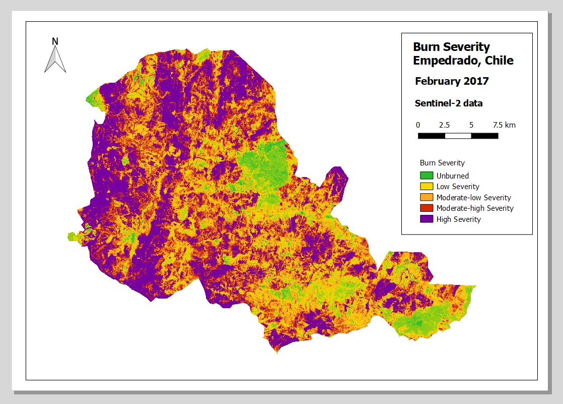
Figure 43. Final Burn Severity Map for Empedrado, Chile, using QGIS.