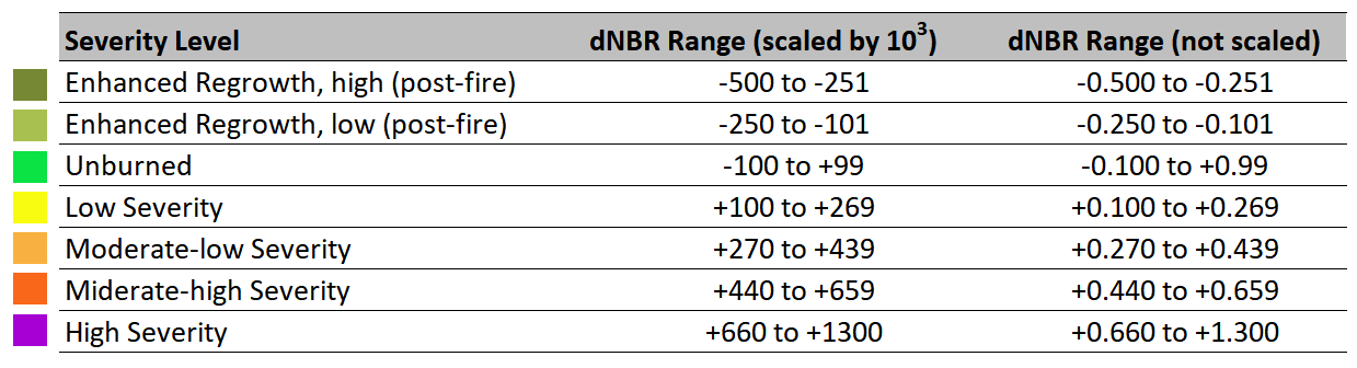
The aim of this step-by-step procedure is the generation of a burn severity map for the assessment of the areas affected by wildfires. The Normalized Burn Ratio (NBR) is used, as it was designed to highlight burned areas and estimate burn severity. It uses near-infrared (NIR) and shortwave-infrared (SWIR) wavelengths. Healthy vegetation before the fire has very high NIR reflectance and a low SWIR response. In contrast, recently burned areas have a low reflectance in the NIR and high reflectance in the SWIR band. More information about the NBR can be found here. The NBR is calculated for images before the fire (pre-fire NBR) and for images after the fire (post-fire NBR) and the post-fire image is subtracted from the pre-fire image to create the differenced (or delta) NBR (dNBR) image. dNBR can be used for burn severity assessment, as areas with higher dNBR values indicate more severe damage whereas areas with negative dNBR values might show increased vegetation productivity. dNBR can be classified according to burn severity ranges proposed by the United States Geological Survey (USGS).
Table 1: Burn severity classes and thresholds proposed by USGS. Color coding established by UN-SPIDER.
Google Earth Engine (GEE) is a powerful web-platform for cloud-based processing of remote sensing data on large scales. The advantage lies in its remarkable computation speed, as processing is outsourced to Google servers. The platform provides a variety of constantly updated datasets, so no download of raw imagery is required. While it is free of charge one still needs to activate their access with a valid Google account. A confirmation usually comes within 2-3 work days. For a quick orientation around the code editor click here.
The code for this Recommended Practice can be imported by following this link.
There you will find detailed comments along with the code line-by-line. Alternatively, you can create a new file in the code editor, download this script and paste it.
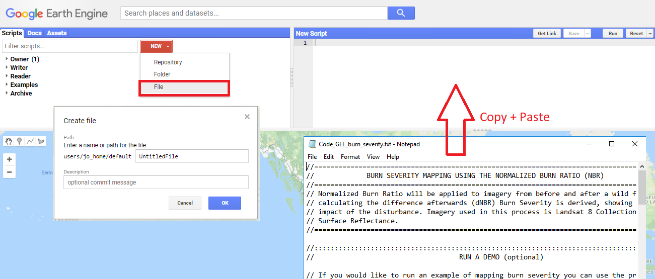
Figure 1: To import the script manually, create a new file and paste the code.
1. Study area selection
In the following section we will present three different ways to specify the location of your study area. This information is necessary to limit the processing extent of the analysis and avoids redundant calculations. Users can upload location information from a file, import country boundaries provided as GEE FeatureCollections or draw an area of interest by hand. These three options as well as all other processing steps are explained in the video tutorial above.
1.1 Shapefiles
Defining the spatial processing extent with an ESRI-Shapefile (.shp) is the most accurate solution. This is recommended, when researching a very destinct study area (e.g. a watershed). Start the import via the 'Assets'-tab in the top left corner. On the 'New'-drop-down menu select 'Table upload', then select your file. Careful: Make sure also to include the .dbf and .shx files, as the shapefile relies on them.
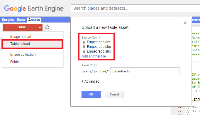
Figure 2: When uploading, include all components of a shapefile: .shp, .shx and .dbf.
Uploading files usually takes a few minutes. You can observe the progress in the 'Tasks'-tab on the top right. Once the 'Asset ingestion'-task is completed (turns blue) you can import the shape to the script. Under 'Assets' click the 'Import'-button so the table is listed in the imports section. In order for the script to recognize this new table, rename it to 'geometry'.
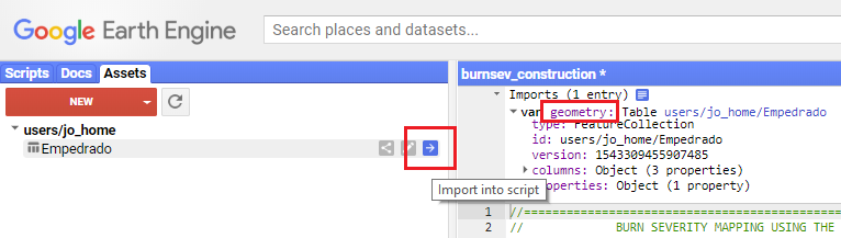
Figure 3: Import the table after uploading and rename it to 'geometry'.
1.2 Built-in Features
GEE so far provides a very limited amount of shapes like administrative boundaries. If one seeks to perform this analysis on country level though, there is a suitable data set provided that contains simplified features. In GEE, search for 'LSIB' or 'International Boundaries'. The FeatureCollection can be imported using its ID ('USDOS/LSIB_SIMPLE/2017'). Select a specific country by filtering the collection by FIPS country code. Here is an example for Costa Rica ('CS'):
var geometry = ee.FeatureCollection('USDOS/LSIB_SIMPLE/2017').filterMetadata('country_co', 'equals', 'CS');
Paste this lines of code at the top of your script and make sure this is the only geometry variable in the script. Replace 'CS' with a country code of your choice.
1.3 Hand-drawn polygons
Besides uploading or importing location data, study area boundaries can be created interactively. This is the quickest and easiest option, suitable for exploring and testing the script in different regions. The polygon tool can be activated in the top-right corner of the map pane. Vertices are created with left clicks and the polygon is completed by double-clicking. A geometry can consist of more than one polygon. Press 'Exit' once you are done setting up your study area. The geometry will be listed under 'Imports' at the top of the script.

Figure 4: Creating a geometry by hand is often the quickest and easiest way in GEE.
2. Time frame
Besides the area of interest, the user is requested to define pre- and post-fire time periods. By setting periods, not single dates, the user allows for the selection of more than one scene per tile, which can later help to find the 'least common denominator' regarding cloud cover. Also, as e.g. Landsat imagery is acquired every 16 days for each point on the globe, providing a time period ensures the detection of such imagery. However, setting longer time periods can have its disadvantages. Refer to the 'limitations' paragraph for more detailed information.
3. Imagery
3.1 GEE ImageCollections
One major advantage of GEE is the accessibility of global time series data in the form of ImageCollections. These are already loaded on Google's servers and do not require much pre-processing. ImageCollections have an ID (e.g. LANDSAT/LC08/C01/T1_SR) and contain a certain type or quality of data. Reading from the ID above, this collection contains Landsat 8 surface reflectance (SR) data from collection one (C01), tier one (T1). ImageCollections can be reduced by applying filters on the region, the date of acquisition or other metadata-filters (e.g. cloud-cover). The GEE code provided in this Recommended Practice prints filtered ImageCollections to the console where they can be explored manually.

Figure 6: Catalogue tree with meta data on an image collection.
3.2 Satellite sensor
For the application of Burn Severity Mapping there are two satellite data collections availible: Landsat 8 and Sentinel-2. The user can chose from these two options. For decision support, a brief overview of satellite data characteristics can be found below.
Table 2: Characteristics of satellite data availible for Burn Severity Mapping in GEE
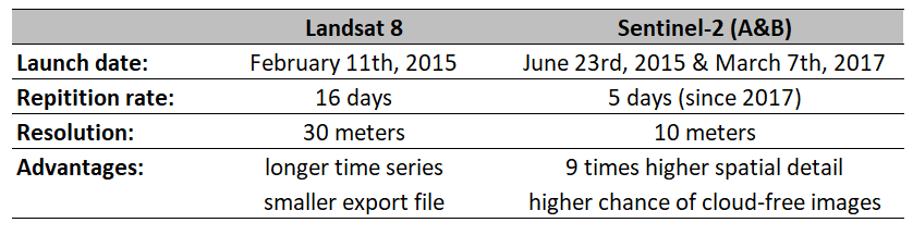
As stated in Table 2, Sentinel-2 data comes with higher spatial detail. This can be an advantage regarding accuracy, expecially in small study areas. The following screenshots compare burn severity results from both sensors and make differences in spatial resolution visible.
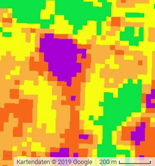

Figure 5: Screenshots of burn severity mapping results from Landsat 8 (left) and Sentinel-2 (right). Sentinel-2s' spatial resolution exceeds Landsat 8's by the factor 9.
3.3 Cloud mask
The script features a cloud-and-snow-masking algorithm based on each sensor's pixel quality assessment band. Thereby, snow, clouds and their shadows are removed from all images of a collection. By mosaicing the masked images a composite with the smallest possible cloud and snow extent is created. Further, mosaics are clipped to the area of interest specified earlier. Although this algorithm has proven to work reliably, caution is advised! Imagery that is mainly occupied by snow, clouds or shadows can sometimes not be masked correctly (see limitations section).

Figure 7: Tunesia's Mediterranean coast between 8th and 30th of April 2018.
Cloud-covered pixels are avoided by compositing all cloud-masked imagery during this time.
Note: This Recommended Practice uses Level-2-processed Landsat 8 imagery. When using e.g. the USGS Earth Explorer for data download, atmospherically corrected imagery (Level 2) can be ordered and is ready for download 2-5 days later. However, raster data sets can not be added to GEE by the user. These data are available only 3-4 weeks after its acquisition date. This time lag plays a major role in terms of disaster and hazard mapping. If you require a more timely solution, choose from one of the other step-by-step-procedures. Landsat 8 was launched 2013 so data is not available prior to that. Sentinel-2 imagery however, is more timely and accessible through GEE few days after its acquisition. The downside is, that Sentinel-2 data is only availible since 2015 (and 2017, respectively).
Statistics
Basic statistics on burned area extent by severity class are implemented in this script. A 'reducer' is employed to count the number of pixels in each class. Besides a simple pixel count, area percentage and area in hectares are listed in the console.
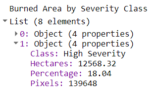
Figure 8: Example of spatial statistics for one burn severity class, ready to explore in the GEE console.
Limitations
Because this is a change detection process, where data from before and after an event are deducted from each other, also non-fire-related changes in the environment can be detected as wild fire damage. Examples include changes in natural vegetation, deforestation and other land cover changes. Snow, clouds and their shadow are masked in one of the pre-processing steps. Nevertheless, masking algorithms sometimes fail to cover e.g. shadows entirely, which can later lead to false detections. The example below shows a post-fire cloud shadow, which has not been masked completely and was then falsely classified as enhanced regrowth.

Figure 9: Cloud shadow (left), not detected by the masking algorithm (center) and falsly classified as regrowth (right).
Slight changes in vegetation (following the natural vegetation period) may also be detected as low severity burn, which is why this class should be treated with special care. Chances of classification errors increase when images are composited over long periods or when distances between these periods get too long. A deliberate trade-off between the amount of available data and irrelevant environmental changes needs to be made.
Therefore knowing the exact time period of the fire prior to this analysis is crucial! By using this information, a suitable time window can be specified at the beginning of the process and errors can be minimized.