You have already downloaded the three required zip files (cf. above under "required datasets"). If not, you will find the links to the data also below.
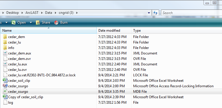
1.1. Unzip cngrid.zip in your working directory. The ArcCatalog-view of the data folder is shown below:
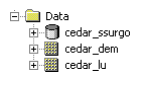
1) cedar_ssurgo is the geodatabase with SSURGO spatial and tabular data for the Cedar Creek area;
2) cedar_dem is the raw 30 DEM for Cedar Creek obtained from USGS and clipped for the study watershed;
3) cedar_lu is the 2001 land cover grid from USGS. All datasets have a common spatial reference (NAD_1983_UTM_16).
1.2. Unzip terrain_geohms.zip in your working directory. The ArcCatalog-view of the data folder is shown below:

1) cedar_dem is the raw 30 DEM for Cedar Creek obtained from USGS and clipped for the study watershed.
Both raster cedar_dem and streams.shp are already assigned a projected coordinate system (NAD_1983_UTM_16).
1.3 Unzip the GeoRASdata.zip file in your working directory. It contains the baxter_tin data required in section 8.2
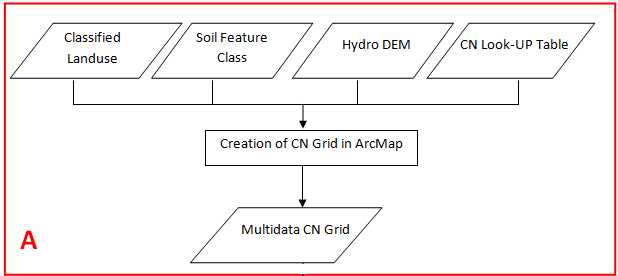
A. Workflow for the Creation of CN Grid in ArcMap
1. Preparing land use data for CN Grid
Open ArcMap. Create a new empty map, and save it as cngrid.mxd (or any other name). Add Spatial Analyst extension and activate it by clicking on Customize --> Extensions…, and checking the box next to Spatial Analyst.
1.1. Add cedar_luse grid to the map document
The grid is added with a unique symbology assigned to cells having identical numbers as you can see below:

These numbers represent a land use class defined according to the USGS land cover institute (LCI). A description of some of the land classes and their associated numbers can be found here.
1.2. Perform the re-classification of classes
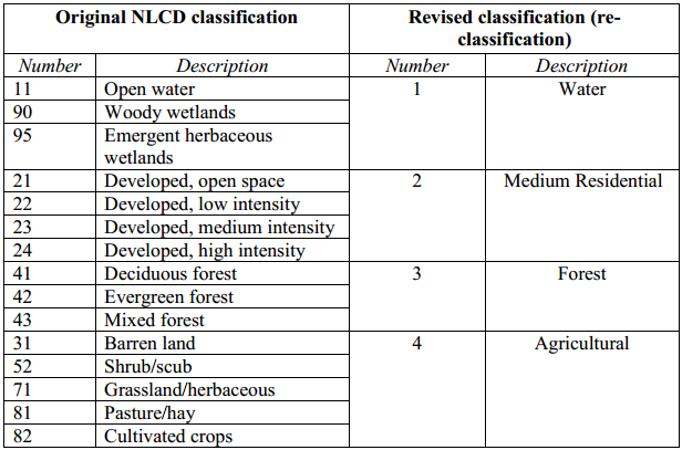
Eventually, we are going to use these land use classes and soil group type, in conjunction with runoff curve numbers (CN), to create the curve number grid. The SCS CN table gives CN for different combinations of land use and soil group. The cedar_lu grid has 15 different categories which you can leave unchanged, or reclassify the grid to reduce the number of land use classes to make the task easier. By opening the attribute table of cedar_lu, you will notice that majority of cells represent grass/crops, followed by forest, developed land, and then water. As these represent the four major classes, we will adequately reclassify cedar_lu. The following table shows how we will accomplish the reclassification of cedar_lu.
To implement the above re-classification, use the Spatial Analyst Tools in Arc Toolbox. Click on Spatial Analyst Tools->Reclass->Reclassify, and then double-click on Reclassify tool.
In the reclassification window, confirm the Input raster is cedar_lu, Reclass field is Value, and then manually assign the new numbers based on the above table as shown below (leave NoData unchanged).

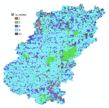
Save the output raster as lu_reclass in your working folder, and click OK. A new grid named lu_reclass will be added to the map as shown below (if you get different colors in symbology is absolutely fine).
1.3. Convert Raster to Polygon
The final step in processing land use data is converting the reclassified land use grid into a polygon feature class which will be merged with soil data later. In ArcToolbox, Click on Conversion Tools->From Raster->Raster to Polygon. Confirm the Input raster is lu_reclass, the Field is Value, output geometry type is Polygon, and save the Output features as landuse_poly.shp in your working directory (this output is saved only as a shapefile without any other options). Click OK.

You can symbolize the new landuse_poly.shp to match with lu_reclass grid or leave it unchanged. Also, you can export landuse_poly.shp to cedar_ssurgo.mdb to keep all the data in a single geodatabase. Save the map document.
The processing of land use data for preparing curve number grid is now done.
2. Preparing Soil data for CN Grid
2.1. Add cedar_soil_clip feature class from spatial feature dataset within cedar_ssurgo.mdb
Create a field named “SoilCode” (type: Text) in cedar_soil_clip. The soil group data are available in the component table (in hydgrp field) so add the component table from cedar_ssurgo.mdb to the map document. Right click on cedar_soil_clip in the ArcMap table of contents, and click on Join and Relates->Join …. Join component table to cedar_soil_clip by using the common mukey field as shown below:

Click OK. You may get a message asking you to index fields. You can respond to this message by selecting either yes or no - it does not matter in this exercise because we will join the table only once. After you create the join, open the attribute table for cedar_soil_clip, and you will see that the fields from component table are now available in cedar_soil_clip feature class. Now populate the SoilCode (or cedar_soil_clip.SoilCode) field in cedar_soil_clip by equating it with component.hydgrp field. With the attribute table open, right click on SoilCode field to open the field calculator and then equate SoilCode to component.hydgrp as shown below:

Click OK. If there are rows in component with “Null” values (which is the case for this dataset), you may get an error message saying the values are too large for the field. Just ignore this message and continue. After the calculations are complete, you should see cedar_soil_clip.SoilCode populated with letters A/B/C/D. Now remove the join and save the map document. Before we proceed, let us deal with
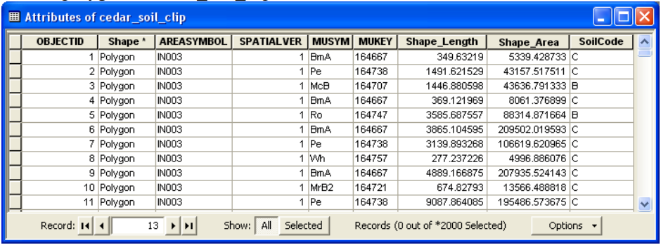
Next create four more fields named PctA, PctB, PctC, and PctD all of type short integer in cedar_soil_clip feature class. For each feature (polygon) in cedar_soil_clip PctA will define what percentage of area within the polygon has soil group A, PctB will define what percentage of area within the polygon will have soil group B and so on. This is critical when we have polygons with more than one soil group (for eg. A-B-A/D would mean that group A, group B and group A/D soils are found in one polygon; A/D would mean the soil behaves as A when drained and as D when not drained, and so on). If we have classifications such as these, we need to define how much area of a polygon is A/B/C/D. For Cedar Creek area we have only one soil group assigned to each polygon so a polygon with soil group “A” will have PctA = 100, PctB = 0, PctC = 0, and PctD = 0. Similarly for a polygon with soil group D, only PctD = 100, and other three Pcts are 0. Now populate PctA, PctB, PctC and PctD based on SoilCode for each polygon. You can select features based on SoilCode and then use field calculator to assign numbers to polygons. Alternatively, you can open the cedar_ssurgo MDB file with a spreadsheet application (e.g. Microsoft Excel, Open Office Calc).
Now open the table cedar_soil_clip and modify the fields PctA, PctB, PctC, and PctD as previously indicated.
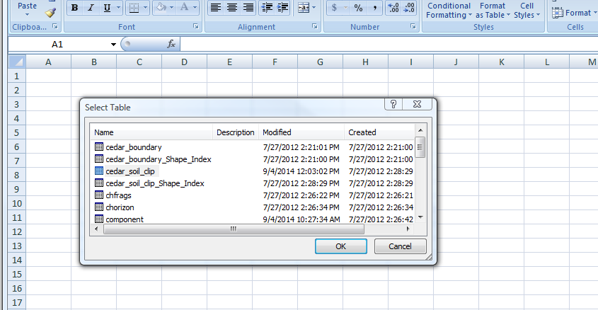
Add the modified table (here indicated with the name cedar_ssurgo$) to the map document
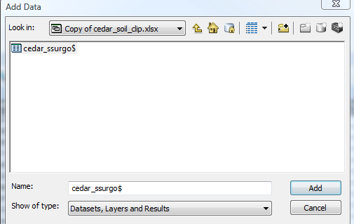
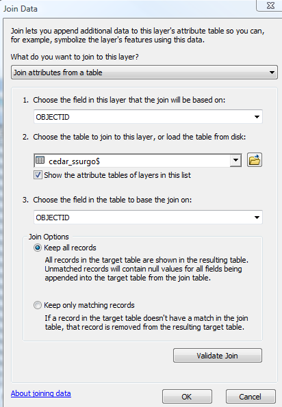
Right click on cedar_soil_clip in the ArcMap table of contents, and click on Join and Relates->Join …. Join cedar_ssurgo$ table to cedar_soil_clip by using the common OBJECTID field as shown below:
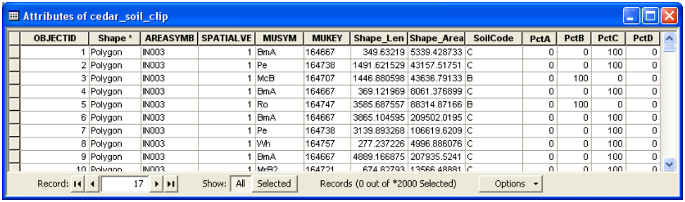
The resulting attribute table should look like below:
The preparation of soil data is done at this point. The next step is to merge/union both soil data and land use data to create polygons that have both soil and land use information. Save the map document.
3. Merging of Soil and Land Use Data
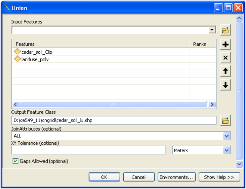
To merge/union soil and landuse data, use the Union tool in ArcToolbox available under Analysis Tools->Overlay. Browse/drag cedar_soil_clip and landuse_poly as input features, name the output feature class as “cedar_soil_lu” in the same geodatabase (cedar_ssurgo.mdb), leave the default options, and click OK (you can change the cluster tolerance to a small number, but this is not necessary).
This process will take few minutes, and the resulting cedar_soil_lu feature class will be added to the map document. Save the map document. The result of union/merge features inherit attributes from both feature classes that are used as input. However, if the outer boundaries of input feature classes do not match exactly, the resulting merged feature class (cedar_soil_lu in this case) usually will have features that will have attributes from only one feature class because the other feature do not exist in this area. These features are usually referred to as “slivers”. If you open the attribute table for cedar_soil_lu, you will find that there are several sliver polygons in this feature class that have attributes only from landuse_poly and the soil attributes are empty, and vice versa as shown below:

In the above table the columns that start with FID_.... give the object ids of features from landuse_poly and cedar_soil_clip. A value of -1 for FID_... means one of the feature classes do have features in that area to union with features from other feature classes. Basically a value of -1 for FID_... means that feature is a sliver polygon. You can also verify this by looking at other 111 fields. For example features that have FID_cedar_soil_clip = -1 have attributes only from landuse_poly and all attributes from cedar_soil_clip = 0.
One way to deal with sliver polygons is to assign missing values to all features. Another way (easiest!) is to just delete them. For this exercise we will take the easy route, but you may want to populate these features for other studies depending on your project needs. Start the Editor. Select all the features that have “FID_...” = -1 and delete them. Save your edits, stop the Editor, and save the map document.
This finishes the processing of spatial data for creating the curve number grid. The next step is to prepare a look-up table that will have curve numbers for different combinations of land uses and soil groups. In this case, we will use SCS curve numbers that are available from literature (SCS reports, or SCS tables from text books). The spatial features in conjunction with the look-up table can then be used to create curve number grid.
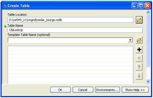
Create a table named “CNLookUp” inside cedar_ssurgo.mdb. In ArcCatalog, select Data Management Tools->Table->Create Table. Once the table is created, create the following fields in it:
[1]. LUValue (type: short integer)
[2]. Description (type: text)
[3]. A (type: short integer)
[4]. B (type: short integer)
[5]. C (type: short integer)
[6]. D (type: short integer)
Now start the Editor to edit the newly created CNLookUp table, and populate it as shown below.
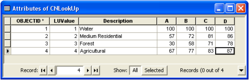
Columns A/B/C/D store curve numbers for corresponding soil groups for each land use category (LUValue). These numbers are obtained from SCS TR55 (1986). Save the edits and stop the Editor. Save the map document.
We will use HEC-GeoHMS to create the curve number grid. Activate the HEC-GeoHMS Project View toolbar in the same way as ArcHydro toolbar. HEC-GeoHMS uses the merged feature class (cedar_soil_lu) and the lookup table (CNLookUp) to create the curve number grid. The format and the field names that we have used in creating the CNLookUp table are consistent with HEC-GeoHMS. Before we proceed, one final step is to create a field in the merged feature class (cedar_soil_lu) named “LandUse” that will have land use category information to link it to CNLookUp table. We already have this information stored in GRIDCODE field, but HEC-GeoHMS looks for this information in LandUse field. So create a field named LandUse (type: short integer), and populate it by equating it to GRIDCODE.
On the HEC-GeoHMS Project View toolbar, click on Utility->Create Parameter Grids. Choose the lookup parameter as Curve Number (which is default) in the next window, Click OK, and then select the inputs for the next window as shown below:
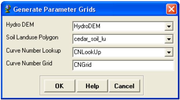
HydroDEM for Hydro DEM, cedar_soil_lu (merged soil and land use) for Curve Number Polygon, CNLookUp table for Curve Number Lookup, and leave the default CNGrid name for the Curve Number Grid.
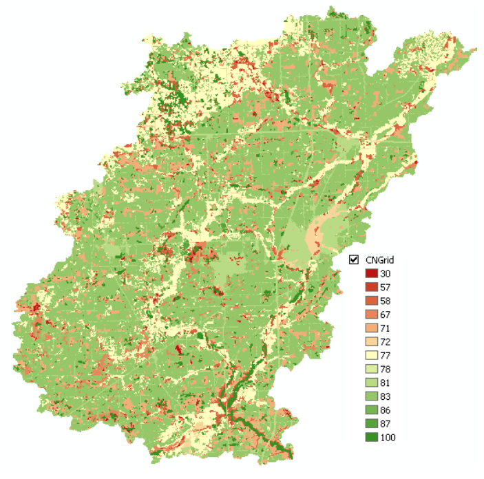
This process takes a while (actually quite a while!). Be patient and CNGrid will be added to your map document. You can change the symbology of the grid to make it look pretty!
You now have a very useful dataset for use in several hydrologic models and studies. Save the map document, and exit ArcMap.
OK. You are done!
B. Hydrological Modeling in ArcHydroTools and HEC-GeoHMS

6. Watershed and Stream Network Delineation using ArcHydro Tools
Open ArcMap. Create a new empty map. Right click on the menu bar to pop up the context menu showing available tools and check the Arc Hydro Tools to add the toolbar to the map document. You should now see the Arc Hydro toolbar added to ArcMap.
The Spatial Analyst Extension has to be activated, by clicking Customize->Extensions…, and checking the box next to Spatial Analyst.
Arc Hydro Terrain Preprocessing should be performed in sequential order. All of the preprocessing must be completed before Watershed Processing functions can be used. DEM reconditioning and filling sinks might not be required depending on the quality of the initial DEM. DEM reconditioning involves modifying the elevation data to be more consistent with the input vector stream network. This implies an assumption that the stream network data are more reliable than the DEM data, so you need to use knowledge of the accuracy and reliability of the data sources when deciding whether to do DEM reconditioning. By doing the DEM reconditioning you can increase the degree of agreement between stream networks delineated from the DEM and the input vector stream networks.
Click on the Add icon to add the raster data. In the dialog box, navigate to the location of the data; select the raster file cedar_dem containing the DEM for Cedar creek and click on the Add button. The added file will then be listed in the Arc Map Table of contents. Similary add stream.shp, and save the map document.
6.1.1. Hydro DEM
6.1.1.1. DEM Reconditioning
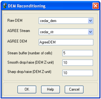
The function needs as input a raw DEM and a linear feature class (like the river network) that both have to be present in the map document. On the ArcHydro toolbar, select Terrain Preprocessing->DEM Manipulation->DEM Reconditioning.
Select the appropriate Raw DEM (cedar_dem) and AGREE stream feature (stream). Set the Agree parameters as shown. You should reduce the Sharp drop/raise parameter to 10 from its default 1000. The output is a reconditioned Agree DEM (default name AgreeDEM).
Click OK on the “…processing successfully completed” message box. Examine the folder where you are working; you will notice that a folder named Layers has been created. This is where ArcHydro will store its grid results.
6.1.1.2. Fill Sinks
This function fills the sinks in a grid. If cells with higher elevation surround a cell, the water is trapped in that cell and cannot flow. The Fill Sinks function modifies the elevation value to eliminate these problems.
On the ArcHydro Toolbar, select Terrain Preprocessing->Data Manipulation->Fill Sinks
Confirm that the input for DEM is AgreeDEM (or your original DEM if Reconditioning was not implemented). The output is the Hydro DEM layer, named by default Fil. This default name can be overwritten. Leave the other options unchanged.
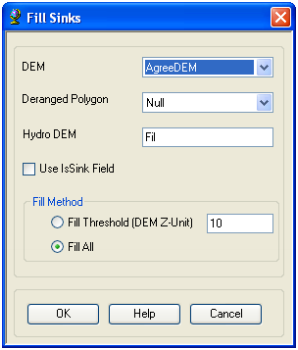
Press OK. Upon successful completion of the process, the Fil layer is added to the map. This process takes a few minutes.
6.1.2. Flow Direction Grid
This function computes the flow direction for a given grid. The values in the cells of the flow direction grid indicate the direction of the steepest descent from that cell.
On the ArcHydro Toolbar, select Terrain Preprocessing->Flow Direction.
Confirm that the input for Hydro DEM is Fil. The output is the Flow Direction Grid, named by default Fdr. This default name can be overwritten.
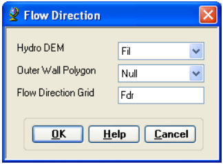
Press OK. Upon successful completion of the process, the flow direction grid Fdr is added to the map.
6.1.3. Flow Accumulation Grid
This function computes the flow accumulation grid that contains the accumulated number of cells upstream of a cell, for each cell in the input grid.
On the ArcHydro toolbar, select Terrain Preprocessing -> Flow Accumulation
Confirm that the input of the Flow Direction Grid is Fdr. The output is the Flow Accumulation Grid having a default name of Fac that can be overwritten.
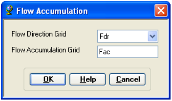
Press OK. Upon successful completion of the process, the flow accumulation grid Fac is added to the map. This process may take several minutes for a large grid! Adjust the symbology of the Flow Accumulation layer Fac to a multiplicatively increasing scale to illustrate the increase of flow accumulation as one descends into the grid flow network.

6.1.4. Stream Definition Grid
On the ArcHydro toolbar, select Terrain Preprocessing -> Stream Definition.
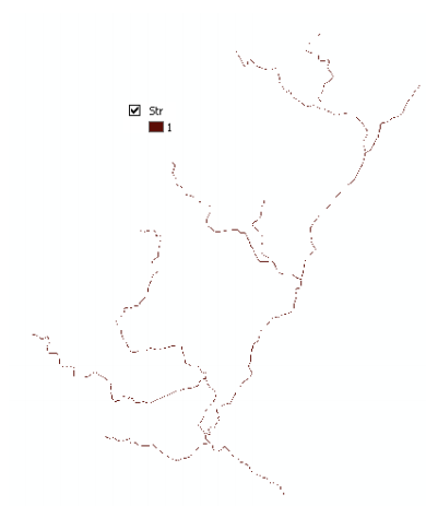
Confirm that the input for the Flow Accumulation Grid is Fac. The output is the Stream Grid named Str, default name that can be overwritten

Objective methods for the selection of the stream delineation threshold to derive the highest resolution network consistent with geomorphological river network properties have been developed and implemented in the TauDEM software (http://www.engineering.usu.edu/dtarb/taudem.). For this exercise, choose 25 km2 as the threshold area, and click OK.
Upon successful completion of the process, the stream grid Str is added to the map. This Str grid contains a value of "1" for all the cells in the input flow accumulation grid (Fac) that have a value greater than the given threshold (26204 as shown in above figure). All other cells in the Stream Grid contain no data. The cells in Str grid with a value of 1 are symbolized with black color to get a stream network as shown below:
6.1.5. Stream Segmentation Grid
This function creates a grid of stream segments that have a unique identification. Either a segment may be a head segment, or it may be defined as a segment between two segment junctions. All the cells in a particular segment have the same grid code that is specific to that segment.
On the ArcHydro toolbar, select Terrain Preprocessing -> Stream Segmentation.

Confirm that Fdr and Str are the inputs for the Flow Direction Grid and the Stream Grid respectively. Unless you are using your sinks for inclusion in the stream network delineation, the sink watershed grid and sink link grid inputs are Null. The output is the stream link grid, with the default name StrLnk that can be overwritten.
Press OK. Upon successful completion of the process, the link grid StrLnk is added to the map. At this point, notice how each link has a separate value. Save the map document.
6.1.6. Catchment Grid Delineation
This function creates a grid in which each cell carries a value (grid code) indicating to which catchment the cell belongs. The value corresponds to the value carried by the stream segment that drains that area, defined in the stream segment link grid.
On the ArcHydro toolbar, select Terrain Preprocessing -> Catchment Grid Delineation.
Confirm that the input to the Flow Direction Grid and Link Grid are Fdr and Lnk respectively. The output is the Catchment Grid layer. Cat is its default name that can be overwritten by the user.
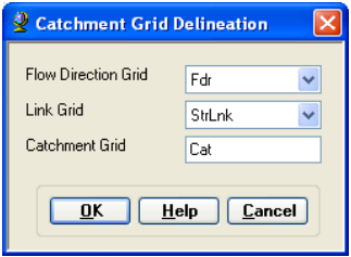
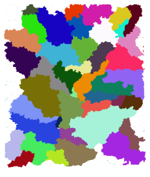
Press OK. Upon successful completion of the process, the Catchment grid Cat is added to the map. If you want, you can recolor the grid with unique values to get a nice display (use properties->symbology).
6.2. Catchment Polygon Processing: Drainage Line, Adjoint Catchment, Drainage Point
The three functions Drainage Line Processing, Adjoint Catchment Processing and Drainage Point Processing convert the raster data developed so far to vector format. The rasters created up to now have all been stored in a folder named Layers. The vector data will be stored in a feature dataset also named Layers within the geodatabase associated with the map document. Unless otherwise specified under APUtilities->Set Target Locations the geodatabase inherits the name of the map document (terrain.mdb in this case) and the folder and feature dataset inherit their names from the active data frame which by default is named Layers.
On the ArcHydro toolbar, select Terrain Preprocessing -> Catchment Polygon Processing. This function converts a catchment grid into a catchment polygon feature.
Confirm that the input to the CatchmentGrid is Cat. The output is the Catchment polygon feature class, having the default name Catchment that can be overwritten.

Press OK. Upon successful completion of the process, the polygon feature class Catchment is added to the map. Open the attribute table of Catchment. Notice that each catchment has a HydroID assigned that is the unique identifier of each catchment within Arc Hydro. Each catchment also has its Length and Area attributes. These quantities are automatically computed when a feature class becomes part of a geodatabase.

6.2.1. Drainage Line
This function converts the input Stream Link grid into a Drainage Line feature class. Each line in the feature class carries the identifier of the catchment in which it resides. On the ArcHydro toolbar, select Terrain Preprocessing -> Drainage Line Processing.
Confirm that the input to Link Grid is Lnk and to Flow Direction Grid Fdr. The output Drainage Line has the default name DrainageLine that can be overwritten.

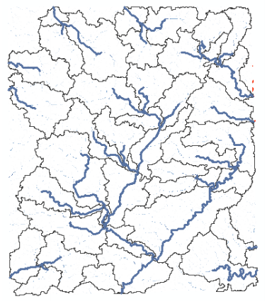
Press OK. Upon successful completion of the process, the linear feature class DrainageLine is added to the map.
6.2.2. Adjoint Catchment
This function generates the aggregated upstream catchments from the Catchment feature class. For each catchment that is not a head catchment, a polygon representing the whole upstream area draining to its inlet point is constructed and stored in a feature class that has an Adjoint Catchment tag. This feature class is used to speed up the point delineation process.
On the ArcHydro toolbar, select Terrain Preprocessing -> Adjoint Catchment Processing
Confirm that the inputs to Drainage Line and Catchment are respectively DrainageLine and Catchment. The output is Adjoint Catchment, with a default name AdjointCatchment that can be overwritten.
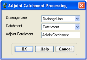
Press OK. Upon successful completion of the process, you will see a message box similar to the one below that will give you a summary of the number of catchments that were aggregated to create the adjoint catchements.
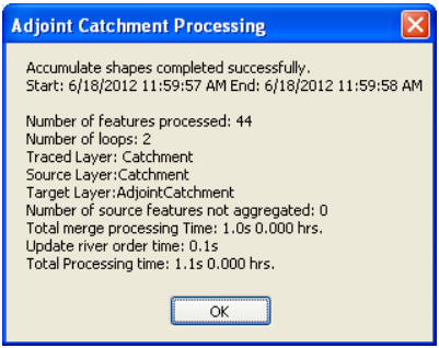
Click OK, and a polygon feature class named AdjointCatchment is added to the map.
6.2.3. Drainage Point
This function allows generating the drainage points associated to the catchments.
On the ArcHydro toolbar, select Terrain Preprocessing -> Drainage Point Processing.
Confirm that the inputs are as below. The output is Drainage Point with the default name DrainagePoint that can be overwritten.

Press OK. Upon successful completion of the process, the point feature class “DrainagePoint” is added to the map.

6.3. Watershed Processing
Arc Hydro toolbar also provides an extensive set of tools for delineating watersheds and subwatersheds. These tools rely on the datasets derived during terrain processing. This part of the exercise will expose you to some of the Watershed Processing functionality in Arc Hydro.
6.3.1. Batch Watershed Delineation
This function delineates the watershed upstream of each point in an input Batch Point feature class.
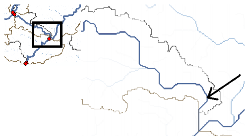
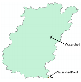
The Arc Hydro tools Batch Point Generation can be used to interactively create the Batch Point feature class. We will use this to locate the outlet of the watershed. Arrange your display so that Fac, Catchment and DrainageLine datasets are visible. Zoom-in near the outlet of the Cedar creek basin (bottom right). The display should look similar to the figure shown below and be zoomed in sufficiently so you can see and click on individual grid cells.
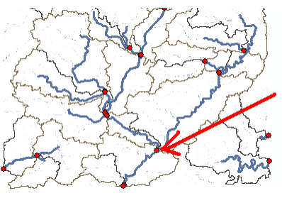
Cedar creek basin and enters St. Joe River. Click on the icon in the Arc Hydro Tools toolbar. Click on the outlet grid cell at the watershed outlet as shown below:
Confirm that the name of the batch point feature class is BatchPoint.
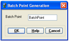
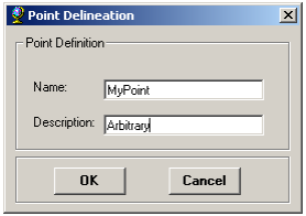
A point is then created at the location of mouse click, and the following form is displayed:

Fill in the fields Name and Description - both are string fields. The BatchDone and SnapOn options can be used to turn on (select 1) or off (select 0) the batch processing and stream snapping for that point. Select the options shown above. The input information is saved in the attribute table of the BatchPoint feature class. Click OK. You should see that a single point feature class has been created comprising the outlet point where you clicked.
When snapping is turned on, if your point is sufficiently near to a drainage line (within around 5 grid cells) then the point will be snapped (i.e. moved) to a nearby drainage line before delineation of the upstream watershed, otherwise the local watershed draining to the point will be delineated.
Note: You can create more points using the same technique at other locations of interest, but for this exercise we will limit our “batch” delineation to only one point (outlet).
To perform a batch watershed delineation: on the Arc Hydro toolbar, select Watershed Processing -> Batch Watershed Delineation.

Confirm that Fdr is the input to Flow Direction Grid, Str to Stream Grid, Catchment to Catchment, AdjointCatchment to AdjointCatchment, and BatchPoint to Batch Point. For output, the Watershed Point is WatershedPoint, and Watershed is Watershed. WatershedPoint and Watershed are default names that can be overwritten.
Press OK. You will get a message indicating that 1 point has been processed.
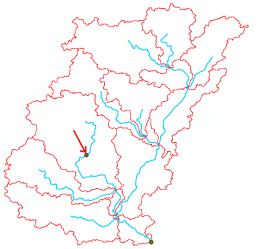
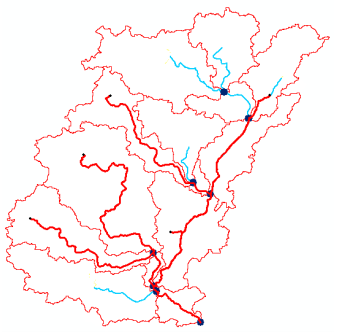
The delineated watersheds for the selected point should correspond closely to the outline of the Cedar creek watershed as shown below (it will match with cedar_dem, and all other derived products):
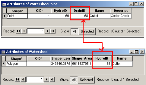
The new watershed is stored in the Watershed feature class and another feature class named WatershedPoint is also added to the map. Open the attribute table of Watershed and WatershedPoint, and you will see that these two are related through HydroID – the DrainID of WatershedPoint is equal to the HydroID of the watershed.
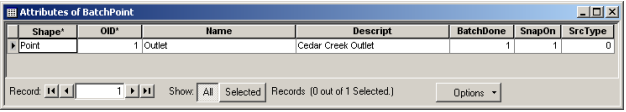
You can also open the attribute table of BatchPoint to see that the value of “BatchDone = 0” that you assigned to this point earlier is now equal to “1”. This tells ArcHydro that the batch processing is done. Due to some reason, if you decide to delineate the watershed for this point again, make sure BatchDone is set to “0”, or else ArcHydro will skip this point.
Delineating Watersheds for existing points (eg. USGS gaging sites)
If you have an existing shapefile or feature class with a set of points that you would like to use instead of interactively creating points, you can do so by using the following guidelines:
- Make sure the points are close enough (within snapping distance) to the corresponding drainage line feature so that they can be snapped to drainage line before delineating the watershed.
- Create two new fields (if already do not exist) in your point shapefile or feature class named BatchDone and SnapOn. Both are Integer type (you can check the field properties of BatchPoint). Also, you can create other fields such as Name, Description etc that exist in BatchPoint, but that is not necessary.
- Make sure all points have “BatchDone” = 0 and “SnapOn” = 1. This will tell ArcHydro that the watersheds for these points are not delineated and the program can snap these points to drainage line before delineating watershed.
- Go to Watershed Processing Batch Watershed Delineation, and make sure you specify the shapefile/feature class that has the batch points for the Batch Point drop-down box (by default the program will use BatchPoint feature class).
Notes:
- Another way to delineate watersheds for existing points is to just load/append these points to the BatchPoint feature class. However, if you want to distinguish your points (for whatever reason) from the default BatchPoint, it is better to just keep them in separate feature class.
- The WatershedPoints that are created as a result of batch watershed delineation will not have any attributes from the USGS gages or any other point feature class that you used in delineating the watersheds. If you want to associate the watershed points with attributes from your point features, you will need to use join and relates or other ways of linking these attributes to watershedpoints. This discussion is beyond the scope of this exercise.
6.3.2. Interactive Point Delineation
An alternative to delineate watersheds when you do not want to use the batch mode (process a group of points simultaneously) to generate the watershed for a single point of interest is the Point Delineation tool.
Click on the Point Delineation icon in the ArcHydro toolbar to activate the tool. Zoom-in to the network and click the mouse (along the drainage line) to create your point of interest.
Fill-in the name and comment as shown below in the form below.
The new point will be added to the WatershedPoint feature class, and the new Watershed will be added to the Watershed feature class.
6.3.3. Batch Subwatershed Delineation
This function delineates subwatersheds for all the points in a selected Point Feature Class. Input to the batch subwatershed delineation function is a point feature class with point locations of interest. In this context a watershed, such as was delineated above is the entire area upstream of a point, while a subwatershed is the area that drains directly to a point of interest excluding any area that is part of another subwatershed. Subwatersheds delineated from a set of points are therefore by definition non overlapping because the watershed draining to a point that is within another watershed is excluded from the subwatershed of the downstream point. On the other hand, watersheds may overlap (For example, the two watersheds in the Watershed feature class overlap with each other). To use the same points that were used for watershed delineation to delineate sub-watersheds, you need to open the attribute table of the points and use the field calculator to set BatchDone = 0 (this will tell Arc Hydro that sub-watersheds are not delineated for these points). To perform sub-watershed delineation, you should use watershed Processing->Batch Subwatershed Delineation option in the ArcHydro toolbar.
6.3.4. Flow Path Tracing
The flow path defines the path of flow from the selected point to the outlet of the catchment following the steepest descent. You can use this option to trace the flow path (the path along which water will flow to the outlet) for any point in the watershed. Click on the Flow Path.
Click on the Tracing icon in the ArcHydro toolbar to activate the tool.
Click with your mouse at any point to determine the flow path. If you select a point along the stream network, the flow path will follow the exact path of the stream.
OK. You are done!
7. Terrain Processing and HEC-GeoHMS Model Development
Open ArcMap. Create a new empty map. Right click on the menu bar to pop up the context menu showing available tools and check the HEC-GeoHMS menu. You should now see the HEC-GeoHMS toolbar added to ArcMap.
Click on the Add icon to add the raster data. In the dialog box, navigate to the location of the data; select the raster file cedar_dem containing the DEM for Cedar creek and click on the Add button. The added file will then be listed in the Arc Map Table of contents. Similary add stream.shp, and save the map document. Save the map document as cedar.mxd.
7.1. Terrain Preprocessing: creation of Slope Grid
Terrain processing involves using the DEM to create a stream network and catchments.
Towards the end of the section 6. you will have the following datasets:
Raster Data:
1. Raw DEM (file name: cedar_dem)
2. HydroDEM ( file name: Fil)
3. Flow Direction Grid ( file name: Fdr)
4. Flow Accumulation Grid ( file name: Fac)
5. Stream Grid ( file name: Str)
6. Stream Link Grid ( file name: StrLnk)
7. Catchment Grid ( file name: Cat)
Vector Data:
1. Catchment Polygons ( file name: Catchment)
2. Drainage Line Polygons ( file name: DrainageLine)
3. Adjoint Catchment Polygons ( file name: AdjointCatchment)
In addition to these datasets, go ahead and also get the slope grid by using the Arc Hydro Toolbar. To create a slope grid using Arc Hydro tools, select Terrain Preprocessing -> Slope.
Confirm that the input as cedar_dem, slope type is percent_rise, and the output will be a slope grid with the default name WshSlopePct that can be overwritten.

This concludes the terrain processing part. What you have produced is a hydrologic skeleton that can now be used to delineate watersheds or sub-watersheds for any given point on delineated stream network. The next part of this tutorial involves delineating a watershed to create a HEC-HMS model using HEC-GeoHMS. Save your map document.
7.2. HEC-HMS Modeling Development using HEC-GeoHMS:
Before you continue, please make sure you have the following datasets in the map document from the previous part.
Raster Data:
1. Raw DEM ( file name: cedar_dem)
2. HydroDEM ( file name: Fil)
3. Flow Direction Grid ( file name: Fdr)
4. Flow Accumulation Grid ( file name: Fac)
5. Stream Grid ( file name: Str)
6. Stream Link Grid ( file name: StrLnk)
7. Catchment Grid ( file name: Cat)
8. Slope Grid (file name: WshSlopePct)
Vector Data:
1. Catchment Polygons ( file name: Catchment)
2. Drainage Line Polygons ( file name: DrainageLine)
3. Adjoint Catchment Polygons ( file name: AdjointCatchment)
Save the map document.
7.2.1. HEC-GeoHMS Project Setup
The HEC-GoeHMS project setup menu has tools for defining the outlet for the watershed, and delineating the watershed for the HEC-HMS project. As multiples HMS basin models can be developed by using the same spatial data, these models are managed by defining two feature classes: ProjectPoint and ProjectArea. Management of models through ProjectPoint and ProjectArea let users see areas for which HMS basin models are already created, and also allow users to re-create models with different stream network threshold. It is also convenient to delete projects and associated HMS files through ProjectPoint and ProjectArea option.
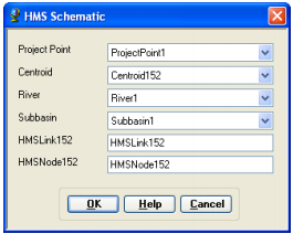
Dataset Setup: Select HMS Project Setup -> Data Management on the HEC-GeoHMS Main View toolbar. Confirm/define the corresponding map layers in the Data Management window as shown below:

Click OK.
To create a new HMS Project, click on Project Setup->Start New Project. Confirm ProjectArea for ProjectArea and ProjectPoint for ProjectPoint, and click OK.

(Note: For some reason, if you get an error message about accuracy/resolution of the data, this has to do with tolerances for x,y,m,z coordinates in your spatial coordinates which you need to fix in ArcCatalog).
This will create ProjectPoint and ProjectArea feature classes. In the next window, provide the following inputs:

If you click on Extraction Method drop-down menu, you will see another option “A new threshold” which will delineate streams based on this new threshold for the new project. For now accept the default original stream definition option. You can write some metadata if you wish,and finally choose the outside MainView Geodatabase for Project Data Location, and browse to your working directory where cedar.mxd is stored. Click OK.
Click OK on the message regarding successful creation of the project. You will see that new feature classes ProjectArea and ProjectPoint are added to ArcMap’s table of contents. These feature classes are added to the same geodatabase cedar.gdb.
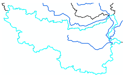
Next Zoom-in to downstream section of the Cedar creek to define the watershed outlet as shown below:
Select the Add Project Points tool on the HEC-GeoHMS toolbar, and click on the downstream outlet area of the cedar creek to define the outlet point as shown below as red dot:
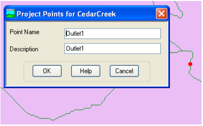
Accept the default Point Name and Description (Outlet), and click OK. This will add a point for the watershed outlet in the ProjectPoint feature class. Save the map document.
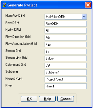
Next, select HMS Project Setup->Generate Project. This will create a mesh (by delineating watershed for the outlet in Project Point), and display a message box asking if you want to create a project for this hatched area as shown below:

(Note: This part could be challenging sometimes. If you face problems in creating Project Area, just delineate a watershed using the point delineation tool in Arc Hydro for the Project Point feature, and load this watershed polygon into ProjectArea feature class. Make sure the HydroID of ProjectArea is same as ProjectID of ProjectPoint. Also you need to make sure the name and description match with each other).
Click Yes on the message box. Next, confirm the layer names for the new project (leave default names for Subbasin, Project Point, River and BasinHeader), and click OK.
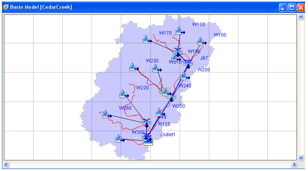
This will create a new folder inside your working folder with the name of the project CedarCreek, and store all the relevant raster, vector and tabular data inside this folder. The raster data are stored in a sub folder with the project name (CedarCreek) inside CedarCreek folder. All vector and tabular data are stored in CedarCreek.mdb. You will also notice that a new data frame (CedarCreek) is added in ArcMap containing data for cedar creek.
You can also play with the contributing area tool to find out contributing area at different points in the cedar creek stream network. With lnk grid active, select the contributing area tool, and click at any point along the stream to know the contributing area.
Save the map document.
7.2.2. Basin Processing
The basin processing menu has features such as revising sub-basin delineations, dividing basins, and merging streams.
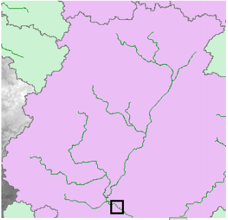
For merging basins, we follow the process that allow us to merges two or more adjacent basins into one. Zoom-in to the area marked in the rectangle below:
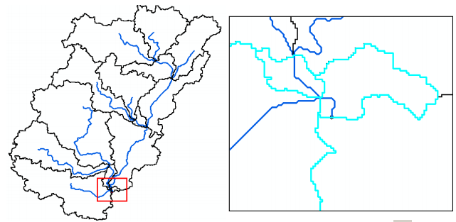
Select the three adjacent basins (shown above) using the standard select tool . Click on Basin Processing-> Basin Merge. You will get a message asking to confirm the merging of selected basins (with basins hatched in background), click Yes. Similarly merge two more sub-basins as shown below:
As a result of this merging, we now have 12 sub-basins and 15 river segments in the project. Save the map document.
For showing the river profile we use the River Profile Tool. It allows displaying the profile of selected river reach(es). If the river slope changes significantly over the reach length, it may be useful to split the river/watershed at such a slope change. Select the River Profile tool , and click on any river segment that you are interested in inspecting. Confirm the layers in the next window, and click OK. This will invoke a dockable window in ArcGIS at the bottom that will display the profile of the selected reach. If you click at a point along the profile, a corresponding point showing its location on the river reach will be added to the map display (shown below as red dot).
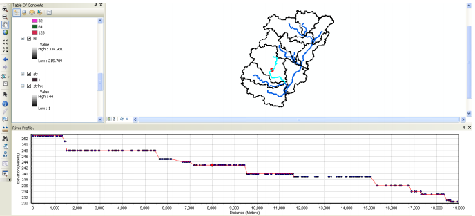
If you want to split the river segment at the selected point, you can just right click on the point inside the dockable window and split the river. If you want to split the sub-basin at the point displayed in the map, you can use the subbasin divide tool, and click at the point displayed on the map. We will not split any river segments in this exercise. Close the dockable window, and save the map document.
7.2.3. Extracting Basin Characteristics: River Lenght, River Slope, Basin Slope, Longest Flow Path, Basin Centroid, Basin Centroid Elevation, Centroidal Longest Flow Path
The basin characteristics menu in the HEC-GeoHMS Project View provide tools for extracting physical characteristics of streams and sub-basins into attribute tables.
The River Lenght tool computes the length of river segments and stores them in RiverLen field. Select Characteristics->River Length. Confirm the input River name, and click OK.

You can check the RiverLen field in the input River1 (or whatever name you have for your input river) feature class is populated. Save the map document.
The River Slope tool computes the slope of the river segments and stores them in Slp field. Select Basin Characteristics->River Slope. Confirm inputs for RawDEM and River, and click OK.
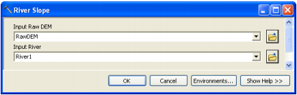
You can check the Slp field in the input River1 (or whatever name you have for your input river) feature class is populated. Fields ElevUP and ElevDS are also populated during this process. Slp = (ElevUP – ElevDS)/RiverLen.
The Basin Slope tool computes average slope for sub-basins using the slope grid and sub-basin polygons. Add wshslopepct (percent slope for watershed) grid to the map document. Select Characteristics->Basin Slope. Confirm the inputs for Subbasin and Slope Grid and click OK.
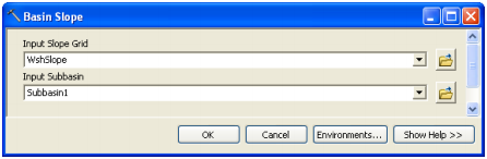
After the computations are complete, the BasinSlope field in the input Subbasin feature class is populated.
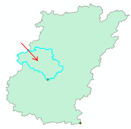
The Longest Flow Path tool will create a feature class with polyline features that will store the longest flow path for each sub-basin. Select Characteristics->Longest Flow Path. Confirm the inputs, and leave the default output name LongestFlowPath unchanged. Click OK.
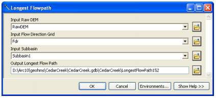
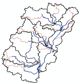
A new feature class storing longest flow path for each sub-basin is created as shown below:
Open the attribute table of Longest Flow Path, and examine its attributes. Close the attribute table, and save the map document.
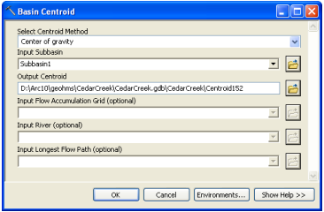
The Basin Centroid tool will create a Centroid point feature class to store the centroid of each sub-basin. Select Characteristics Basin Centroid. Choose the default Center of Gravity Method, input Subbasin, leave the default name for Centroid. Click OK.
(Note: Center of Gravity Method computes the centroid as the center of gravity of the sub basin if it is located within the sub basin. If the Center of Gravity is outside, it is snapped to the closest boundary. Longest Flow Path Method computes the centroid as the center of the longest flow path within the sub basin. The quality of the results by the two methods is a function of the shape of the sub basin and should be evaluated after they are generated.)
A point feature class showing centroid for each sub-basin is added to the map document.
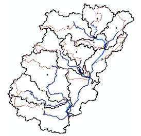
As centroid locations look reasonable, we will accept the center of gravity method results, and proceed. Save the map document.
The Basin Centroid Elevation tool will compute the elevation for each centroid point using the underlying DEM. Select Characteristics->Centroid Elevation Update. Confirm the input DEM and centroid feature class, and click OK.
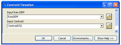
After the computations are complete, open the attribute table of Centroid to examine the Elevation field. The centroid elevation update may be needed when none of the basin centroid methods (center of gravity or longest flow path) provide satisfactory results, and it becomes necessary to edit the Centroid feature class and move the centroids to a more reasonable location manually.
To define the Centroidal Longest Flow Path, select Characteristics->Centroidal Longest Flow Path. Confirm the inputs, and leave the default name for output Centroidal Longest Flow Path, and Click OK.
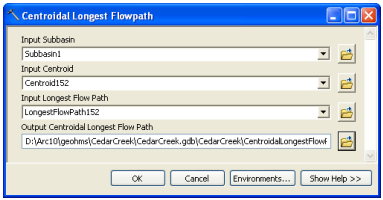
This creates a new polyline feature class showing the flowpath for each centroid point along longest flow path. Save the map document.
7.2.4. HMS Inputs/Parameters: River Auto Name, Basin Auto Name, HMS Units
The hydrologic parameters menu in HEC-GeoHMS provides tools to estimate and assign a number of watershed and stream parameters for use in HMS. These parameters include SCS curve number, time of concentration, channel routing coefficients, etc.
You can specify the methods that HMS should use for transform (rainfall to runoff) and routing (channel routing) using this function. Of course, this can be modified and/or assigned inside HMS.
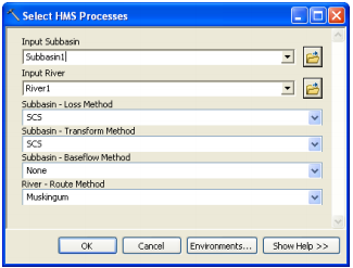
Select Hydrologic Parameters->Select HMS Processes. Confirm input feature classes for Subbasin and River, and click OK. Choose SCS for Loss Method (getting excess rainfall from total rainfall), SCS for Transform Method (for converting excess rainfall to direct runoff), None for Baseflow Type, and Muskingum for Route Method (channel routing). Click OK.
You can open the attribute table of subbasin feature class to see that the subbasin methods are added to LossMet, TransMet, and BaseMet fields, respectively. The Muskingum method is added to RouteMet field in the River feature class. You can treat these methods as tentative which can be changed in HMS model. Save the map document.
7.2.4.1. River Auto Name
The River Auto Name function assigns names to river segments. Select Parameters->River Auto Name. Confirm the input feature class for River, and click OK.

The Name field in the input River feature class is populated with names that have “R###” format, where “R” stands for river/reach “###” is an integer.
7.2.4.2. Basin Auto Name
The Basin Auto Name function assigns names to sub-basins. Select Parameters->Basin Auto Name. Confirm the input feature class for sub-basin, and click OK.

Like river names, the Name field in the input Subbasin feature class is populated with names that have “W###” format, where “W” stands for watershed, and “###” is an integer. Save the map document.
Depending on the method (HMS process) you intend to use for your HMS model, each sub-basin must have parameters such as SCS curve number for SCS method and initial loss constant, etc. These parameters are assigned using Subbasin Parameters option. This function overlays subbasins over grids and compute average value for each basin. We will explore only those parameters that do not require additional datasets or information.
Add cngrid (curve number grid) from Layers folder to the map document. Select Hydrologic Parameters->Subbasin Parameters. You will get a menu of parameters that you can assign. Uncheck all parameters and check BasinCN as shown below, and Click OK.

Confirm the inputs for Subbasin and Curve Number Grid, and click OK.
After the computations are complete, you can open the attribute table for subbasin, and see that a field named BasinCN is populated with average curve number for each sub-basin. Close the attribute table, and save the map document.
(Note: We will skip parameters associated with computing rainfall as these numbers should come from detailed analysis of the watershed. However, if you are interested, you can explore these functions because you have all the necessary data for their execution.)
The CN Lag Method function computes basin lag in hours (weighted time of concentration or time from the center of mass of excess rainfall hyetograph to the peak of runoff hydrograph) using the NRCS National Engineering Handbook (1972) curve number method. Select Hydrologic Parameters->CN Lag Method. This function populates the BasinLag field in the subbasin feature class with numbers that represent basin lag time in hours. Save the map document. Take a look at attribute tables of River and Subbasin feature class to see what fields are populated, and what they mean in hydrologic modeling.
Confirm the inputs for Subbasin and Curve Number Grid, and click OK.
7.2.4.3. Map to HMS Units
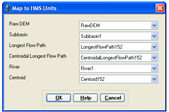
This tool is used to convert units. Click on HMS->Map to HMS Units. Confirm the input files, and click OK.
(Note: Due to some unknown reasons, if you get an error message at this point saying field cannot be added to a layer, save the map document, exit ArcMap and open the document, and try again).
In the next window, choose English units (default) from the drop-down menu, and click OK.

After this process is complete, you will see new fields in both River and Subbasin feature classes that will have fields ending with “_HMS” to indicate these fields store attributes in the specified HMS units (English in this case). All fields that store lengths and areas will have corresponding “_HMS” fields as a result of this conversion.
7.2.5. Check Data
This tool will verify all the input datasets. Select HMS->Check Data. Confirm the input datasets to be checked, and click OK.
You should get a message after the data check saying the check data is completed successfully as shown below.
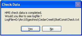
You can also look at the log file and make sure there are no errors in the data by scrolling to the bottom of the log file as shown below:

If you get problems in any of the above four categories (names, containment, connectivity and relevance), you can look at the log file to identify the problem, and fix them by yourself. This version of HecGeoHMS apparently gives error with river connectivity even if the rivers are well connected. Therefore, check the data carefully, and if you think everything is OK, ignore the errors (if you get any for connectivity) and proceed.
7.2.6. HMS Schematic
This tool creates a GIS representation of the hydrologic system using a schematic network with basin elements (nodes/links or junctions/edges) and their connectivity. Select HMS->HMS Schematic. Confirm the inputs, and click OK.
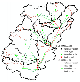
Two new feature classes HMS Link and HMSNode will be added to the map document.
After the schematic is created, you can get a feel of how this model will look like in HEC-HMS by toggling/switching between regular and HMS legend. Select HMS->Toggle HMS Legend->HMS Legend.
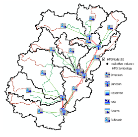
You can keep whatever legend you like. Save the map document.
7.2.7. Add Coordinates
This tool attaches geographic coordinates to features in HMSLink and HMSNode feature classes. This is useful for exporting the schematic to other models or programs without loosing the geospatial information. Select HMS->Add Coordinates. Confirm the input files, and click OK.
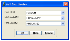
The geographic coordinates including the “z” coordinate for nodes are stored as attributes (CanvasX, CanvasY, and Elevation) in HMSLink and HMSNode feature classes.
7.2.8. Prepare Data for Model Export
Select HMS->Prepare Data for Model Export. Confirm the input Subbasin and River files, and click OK.
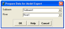
This function allows preparing subbasin and river features for export.
7.2.9. Background Shape File
Select HMS->Background Shape File. This function captures the geographic information (x,y) of the subbasin boundaries and stream alignments in a text file that can be read and displayed within HMS. Two shapefiles: one for river and one for sub-basin are created in the project folder. Click OK on the process completion message box.
7.2.10. Basin Model
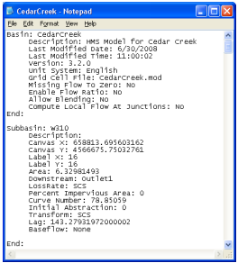
Select HMS->Basin Model File. This function will export the information on hydrologic elements (nodes and links), their connectivity and related geographic information to a text file with .basin extension. The output file CedarCreek.basin (project name with .basin extension) is created in the project folder. Click OK on the process completion message box.
You can also open the .basin file using Notepad and examine its contents.
7.2.11. Meteorologic Model
We do not have any meteorologic data (temperature, rainfall etc) at this point. We will only create an empty file that we can populate inside HMS. Select HMS->Met Model File->Specified Hyetograph. The output file CedarCreek.met (project name with .met extension) is created in the project folder. Click OK on the process completion message box.
You can also open the .met file using Notepad and examine its contents.
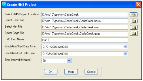
7.2.12. HMS Project
This function copies all the project specific files that you have created (.met, .map, and .met) to a specified directory, and creates a .hms file that will contain information on other files for input to HMS. Select HMS->Create HMS Project. Provide locations for all files. Even if we did not create a gage file, there will be a gage file created when the met model file is created. Give some name for the Run, and leave the default information for time and time interval unchanged. This can be changed in HEC-HMS based on the event you will simulate. Click OK.
If a .hms file already exist in that folder, you may get a message asking you to overwrite or not. After you respond to that message a project file report will be displayed as shown below:
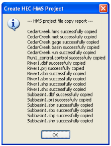
This set of files displayed in project report defines the HMS project that you can open and manipulate in HMS directly without interacting with GIS. Typically, you will have to modify meteorologic and basin files to reflect field conditions before actually running the HMS model. Close the report. Save the map document.
7.3. Opening the HMS Model
This section briefly explains how to interface or open the project files created by GeoHMS using HMS.
Open HEC-HMS, and select File->Open. Browse to CedarCreek.hms file, and click Open. You will see that two folders: Basin Models and Meteorologic Models will be added to the Watershed Explorer (window on top-left) in HEC-HMS. Expand the Basin Models folder and click on CedarCreek. This will display the Cedar creek schematic. Click on View->Background Map, and then add the river and basin shapefiles to see the watershed as shown below.
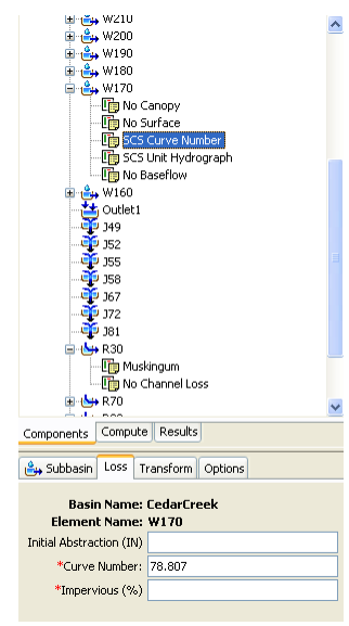
If you expand the CedarCreek basin in watershed explorer, you will see the list of junctions, reaches and subbasins. You can click on any reach and see its associated methods. For example, when you click on a Reach (R##), you will see that Muskingum routing method is associated with it. Similarly, if you click on a Watershed (W##), you will see SCS Curve Number (for abstractions) and SCS Unit Hydrograph (for runoff calculations) are associated with it. Again, if you click on SCS Curve Number, you will see corresponding parameters in the Component Window as shown below. All this information, which is now independent of GIS, is extracted from attributes that we created in HEC-GeoHMS.
Manipulating data in HMS, populating the Meteorologic file, and running the model is beyond the scope of this tutorial. Save your HMS project.
C. Hydraulic Modeling Workflow
8. HECGeo-RAS: Hydraulic Modelling
Install HEC GeoRAS onto your computer, Open Arc map click the customize menu (Scrolldown the list to see “Customize") In the Customize dialog that appears, check the Hec Geo RAS Tools box.
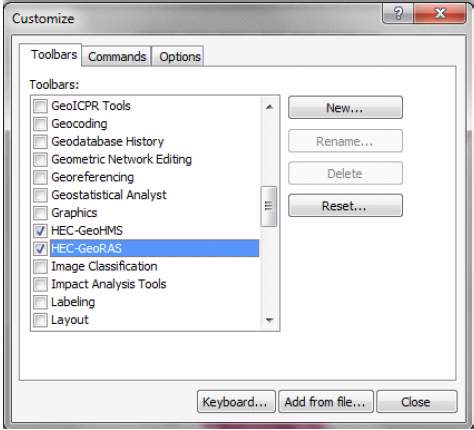
You should be able to see a Hec Geo RAS tools menu added.
8.1. Data Setup
The only essential dataset required for HEC-GeoRAS is the terrain data (TIN or DEM). Additional datasets that may be useful are aerial photograph(s) and land use information. The TIN or DEM may derived from a contour map. Note: hydraulic modelling requires data with higher/better resolution as compared to hydrological modelling in HEC Geo HMS.
8.2. Setting up Analysis Environment for HEC-GeoRAS
Using GIS for hydrologic/hydraulic modeling usually involves three steps: 1) preprocessing of data, 2) model execution, and 3) post-processing/visualization of results. It is common to use a single map document to handle a single project, but this ends up with too many feature classes/layers in a single map. It is then cumbersome to find out which feature classes were used during pre-processing, and which feature classes contain results for visualization. To avoid this confusion, HEC-GeoRAS uses separate data frames to organize pre- and post-processing data.
To create a geometry file, you need terrain (elevation) data. Click on Add button in ArcMap, and browse to baxter_tin to add the terrain to the map document (cf. section on "Required Datasets" above regarding the download of the dataset). You must have the same coordinate system for all the data and data frames used for this tutorial (or any GeoRAS project). Because baxter_tin already has a projected coordinate system, it is applied to the BaxterGeometry data frame. You can check this by right-clicking on the data frame and looking at its properties.
8.3. Creating RAS layers

In the Create All Layers window, accept the default names, and click OK. HEC-GeoRAS creates a geodatabase in the same folder where the map document is saved, gives the name of the map document to the geodatabase baxter_georas.mdb, in this case), and stores all the feature classes/RAS layers in this geodatabase.
After creating RAS layers, these are added to the map document with a pre-assigned symbology.Since these layers are empty, our task is to populate some or all of these layers depending on our project needs, and then create a HEC-RAS geometry file.
8.4. Creating a river centerline
Let us first start with river centerline. The river centerline is used to establish the river reach network for HEC-RAS. The river has different tributaries as shown below.
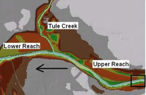
We will create/digitize one feature for each reach approximately following the center of the river, and aligned in the direction of flow. Zoom-in to the most upstream part of the ceedar creek tributaries.
To create the river centerline (in River feature class), start editing, and choose Create New Feature as the Task, and River as the Target as shown below:
Using the Sketch tool (highlighted above), start digitizing the river centerline from upstream to downstream until you reach the intersection with Tule Creek tributary. To digitize the upper Baxter River reach, click in the direction of flow and double click when done (at intersection with Tule Tributary). If you need to pan, click the pan tool, pan through the map and then continue by clicking the sketch tool (do not double-click until you reach the junction). After finishing digitizing the upper Baxter Reach, save the edits. Before you start digitizing the Tule Creek tributary, modify some editing options. Click on Editor->Snapping, and check the End box next to River.
We are modifying the editing environment because when we digitize the Tule tributary we want its downstream end coincide with the downstream end of the upper Baxter Reach. Close the snapping box, and then start digitizing the Tule Tributary from its upstream end towards the junction with the Baxter River. When you come close to the junction, zoom-in, and you will notice that the tool will automatically try to snap (or hug!) to the downstream end of the upper Baxter Reach. Double click at this point to finish digitizing the Tule Tributary. Save edits. Finally, digitize the lower Baxter reach from junction with the Tule Tributary to the most downstream end of the Baxter River. Again make sure you snap the starting point with the common end points of Upper Baxter Reach and Tule Tributary. Save edits, and stop editing. (Snapping of all the reaches at the junction is necessary for connectivity and creating HEC-RAS junction so make sure the three reaches are snapped correctly).
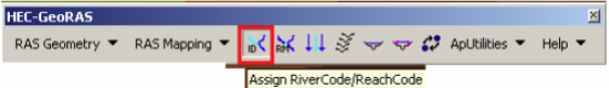
After the reaches are digitized, the next task is to name them. Each river in HEC-RAS must have a unique river name, and each reach within a river must have a unique reach name. We can treat the main stem of the Baxter River as one river and the Tributary as the second river. To assign names to reaches, click on Assign RiverCode/ReachCode button to activate it as shown below:
With the button active, click on the upper Baxter River reach. You will see the reach will get selected, invoking the following window:
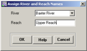
Assign the River and Reach name as Baxter River and Upper Reach, respectively, and click OK. Click on the tributary reach, and use Tule Creek and Tributary for River and Reach name, respectively. For lower Baxter river, use Baxter River and Lower Reach for River and Reach name, respectively.
Now open the attribute table of River featureclass, and you will see that the information you just provided on river and reach names is entered as feature attributes as shown below:
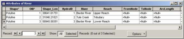
Also note that there are still some unpopulated attributes in the River feature class (FromNode, ToNode, etc.).
Before we move forward let us make sure that the reaches we just created are connected, and populate the remaining attributes of the River feature class. Click on RAS Geometry->Stream Centerline Attributes->Topology.

Confirm River for Stream Centerline and baxter_tin for Terrian TIN, and click OK. This function will populate the FromNode and ToNode attribute of the River feature class. Next, click on RAS Geometry->Stream Centerline Attributes->Lengths/Stations. This will populate the remaining attributes. Now open the attribute table for River, and understand the meaning of each attribute.

HydroID is a unique number for a given feature in a geodatabase. The River and Reach attributes contain unique names for rivers and reaches, respectively. The FromNode and ToNode attributes define the connectivity between reaches. ArcLength is the actual length of the reach in map units, and is equal to Shape_Length. In HEC-RAS, distances are represented using station numbers measured from downstream to upstream. For example, each river has a station number of zero at the downstream end, and is equal to the length of the river at the upstream end. Since we have only one reach for Tule Creek tributary the FromSta attribute is zero and the ToSta attribute is equal to the ArcLength. Since the Baxter River has two reaches, the FromSta attribute for Upper Reach = ToSta attribute of lower reach, and the ToSta attribute for upper reach is the sum of ArcLengths for the upper and lower reach. Close the attribute table, and save the map document.
8.5. Creating River Banks
Bank lines are used to distinguish the main channel from the overbank floodplain areas. Information related to bank locations is used to assign different properties for crosssections. For example, compared to the main channel, overbank areas are assigned higher values of Manning’s n to account for more roughness caused by vegetation. Creating bank lines is similar to creating the channel centerline, but there are no specific guidelines with regard to line orientation and connectivity - they can be digitized either along the flow direction or against the flow direction, or may be continuous or broken.
To create the channel centerline (in Banks feature class), start editing, and choose Create New Feature as the Task, and Banks as the Target as shown below:
Although there are no specific guidelines for digitizing banks, to be consistent, follow these guidelines: 1) start from the upstream end; 2) looking downstream, digitize the left bank first and then the right bank.
Digitize banks for all three reaches and save the edits and the map document.
8.6. Creating the Flowpath Layer
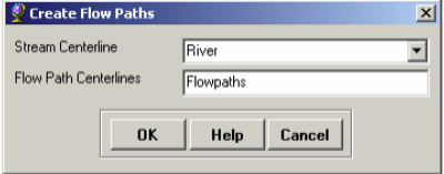
The flowpath layer contains three types of lines: centerline, left overbank, and right overbank. The flowpath lines are used to determine the downstream reach lengths between cross-sections in the main channel and over bank areas. If the river centerline that we created earlier lie approximately in the center of the main channel (which it does), it can be used as the flow path centerline. Click on RAS GeometryCreate RAS LayersFlow Path Centerlines Click Yes on the message box that asks if you want to use the stream centerline to create the flow path centerline. Confirm River for Stream Centerline and Flowpaths for Flow Path Centerlines, and click OK.
To create the left and right flow paths (in Flowpaths feature class), start editing, and choose Create New Feature as the Task, and Flowpaths as the Target as shown below:
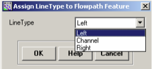
Use the sketch tool to create flowpaths. The left and right flowpaths must be digitized within the floodplain in the downstream direction. These lines are used to compute distances between cross-sections in the over bank areas. Again, to be consistent, looking downstream first digitize the left flowpath followed by the right flowpath for each reach. After digitizing, save the edits and stop editing. Now label the flowpaths by using the Assign LineType button. Click on the button (notice the change in cursor), and then click on one of the flow paths (left or right, looking downstream), and name the flow path accordingly as shown below:
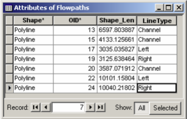
Label all flow paths, and confirm this by opening the attribute table of the Flowpaths feature class. The LineType field must have data for each row if all flowpaths are labeled.
8.7. Creating cross sections
Cross-sections are one of the key inputs to HEC-RAS. Cross-section cutlines are used to extract the elevation data from the terrain to create a ground profile across channel flow. The intersection of cutlines with other RAS layers such as centerline and flow path lines are used to compute HEC-RAS attributes such as bank stations (locations that separate main channel from the floodplain), downstream reach lengths (distance between crosssections) and Mannings number. Therefore, creating adequate number of cross-sections to produce a good representation of channel bed and floodplain is critical.
Certain guidelines must be followed in creating cross-section cutlines: (1) they are digitized perpendicular to the direction of flow; (2) must span over the entire flood extent to be modeled; and (3) always digitized from left to right (looking downstream).
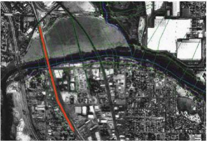
Even though it is not required, but it is a good practice to maintain a consistent spacing between cross sections. In addition, if you come across a structure (eg. bridge/culvert) along the channel, make sure you define one cross-section each on the upstream and downstream of this structure. Structures can be identified by using the aerial photograph provided with the tutorial dataset. For example, we will use one bridge location in this exercise just downstream of the junction with tributary as shown below (bridge location is shown in red):
To create cross-section cutlines (in XSCutlines feature class), start editing, and choose Create New Feature as the Task, and XSCutlines as the Target as shown below:
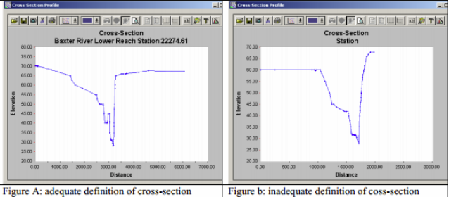
Follow the above guidelines and digitize cross-sections using the sketch tool. While digitizing, make sure that each cross-section is wide enough to cover the floodplain. This can be done using the cross-sections profile tool. Click on the profile tool, and then click on the cross-section to view the profile. For example, if you get a cross-section profile shown in Figure A below, then there is no need to edit the cross-section, but if you get a cross-section as shown in Figure B below, then the cross-section needs editing. (Note: This tool stops the edit session so you will have to start the edit session every time after viewing the cross-section profile).
After digitizing the cross-sections, save the edits and stop editing. The next step is to add HEC-RAS attributes to these cutlines. We will add Reach/River name, station number along the centerline, bank stations and downstream reach lengths. Since all these attributes are based on the intersection of cross-sections with other layers, make sure each cross-section intersects with the centerline and overbank flow paths to avoid error messages.
Click on RAS Geometry->XS Cut Line Attributes->River/Reach Names. This tool uses the River and Reach attributes of the centerline, and copy them to the XS Cutlines. Next, click on RAS Geometry->XS Cut Line Attributes->Stationing. This tool will assign station number (distance from each cross-section to the downstream end of the river) to each cross-section cutline. Next, click on RAS Geometry->XS Cut Line Attributes-> Bank Stations. Confirm XSCutlines for XS Cut Lines, and Banks for Bank Lines, and click OK.

This tool assigns bank stations (distance from the starting point on the XS Cutline to the left and right bank, looking downstream) to each cross-section cutline. Finally, click on RAS Geometry->XS Cut Line Attributes->Downstream Reach Lengths. This tool assigns distances to the next downstream cross-section based on flow paths.
The cross-section cutlines are 2D lines with no elevation information associated with them (Polyline). When you used the profile tool earlier to view the cross-section profile, the program used the underlying terrain to extract the elevations along the cutline. You can convert 2D cutlines into 3D by clicking RAS Geometry->XS Cut Line Attributes->Elevation. Confirm XSCutlines for XS Cut Lines, and baxter_tin for Terrian TIN. The new 3D lines (XS Cut Lines Profiles) will be stored in the XSCutLines3D feature class. Click OK.
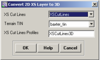
After this process is finished, open the attribute table of XSCutLines3D feature class and see that the shape of this feature class is now PolylineZ.
8.8. Creating Bridges and Culverts
After creating cross-sections, the next step is to define bridges, culverts and other structure along the river. Since we used aerial photograph while defining the crosssections, our job of locating the bridge is done. To create bridges/culverts (in Bridges feature class), start editing, and choose Create New Feature as the Task, and Bridges as the Target as shown below:
A bridge or culvert is treated similar to a cross-section so the same criteria used for creating cross-sections must be used for bridge/culverts. Using the sketch tool on the editor toolbar, the digitize bridge location just downstream of the tributary junction. While digitizing the bridge, make use of the terrain model to make sure the bridge/road centerline fall on the high ground. Save your edits and stop editing.
Close the attribute table, save edits and stop editing.
Similar to cross-sections, the Bridges feature class stores 2D polylines, you can make them 3D by clicking RAS Geometry->Bridge/Culverts->Elevations to create a new 3D Bridges feature class. Confirm Bridges for Bridges/Culverts, baxter_tin for Terrain, Bridges 3D for Bridges/Culverts Profiles, and Click OK.
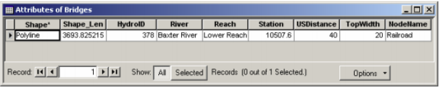
After digitizing bridges/culverts, you need to assign attributes such as River/Reach name and station number to these features. Click on RAS Geometry-> Bridge/Culverts-> River/Reach Names to assign river/reach names. Next click on RAS Geometry->Bridge/Culverts->Stationing to assign station numbers. Besides these attributes, you must enter additional information about the bridge(s) such as the name and width in its attribute table as shown below.

A new feature class (Bridges3D) will be created. You can check it is PolylineZ by opening its attribute table.
8.9. Creating ineffective flow areas
Ineffective flow areas are used to identify non-conveyance areas (areas with water but no flow/zero velocity) of the floodplain. For example, areas behind bridge abutments representing contraction and expansion zones can be considered as ineffective flow areas. To define ineffective areas (in IneffAreas feature class), start editing, and choose Create New Feature as the Task, and IneffAreas as the Target as shown below:

HEC-RAS does not store all information about ineffective areas. Instead only the information where the ineffective area may interfere with cross-sections/flow is stored. To extract the position and elevation at points where these ineffective areas intersect with cross-sections, click on RAS Geometry->Ineffective Flow Areas->Position. Leave the default feature classes for IneffectiveAreas, XS Cut Lines, and Terrain unchanged. The position of ineffective areas will be stored in a new table named IneffectivePositions. Leave current user elevations unchecked, and Click OK.

Open the attributes of the IneffectivePositions table (shown below) to understand how this information is stored.

IA2DID is the HydroID of the ineffective flow area, XS2DID is the HydroID of the intersecting cross-section, BeginFrac and EndFrac are the relative positions of the first and last intersecting points (looking downstream) of the ineffective area with the crosssection. BegElev and EndElev are the elevations of the first and last intersecting points of the ineffective area with the crosssection. Since you left the UserElev box unchecked there are no values in this field.
8.10. Creating Obstructions
Obstructions represent blocked flow areas (areas with no water and no flow). For example, buildings in the floodplain and levees are considered obstructions. We can add blocked obstructions to our study by using building locations in the aerial photograph.
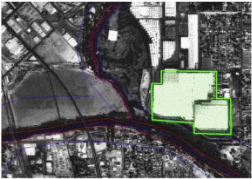
To define blocked obstructions (in BlockedObs feature class), start editing, and choose Create New Feature as the Task, and BlockedObs as the Target as shown below:
Use the Sketch tool to define the blocked obstruction, save edits and stop editing. Similar to Ineffective flow areas, the positions and elevations of the intersection of this obstruction with cross-sections needs to be stored in a table. Click on RAS Geometry->Blocked Obstructions-> Positions. Leave the default values in the Blocked Obstructions window, and click OK. You will notice that a new table (BlockedPositions) will be added to the map document, and its content are identical to IneffectivePositions table.
8.11. Assigning Manning’s n to cross-sections
The final task before exporting the GIS data to HEC-RAS geometry file is assigning Manning’s number value to individual cross-sections. In HEC-GeoRAS, this is accomplished by using a land use feature class with Manning’s n stored for different land use types. Ideally you will store this information in the LandUse feature class added to the map.

The land use table must have a descriptive field identifying landuse type, which is LUCode in this case, and a field for corresponding Manning’s n values. In addition, HEC-GeoRAS requires the land use polygons to be non multi-part features (a multipart feature has multiple geometries in the same feature). The issue of non multi-part features is taken care of for the tutorial dataset.
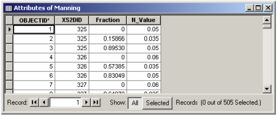
To assign Manning’s n to cross-sections, click on RAS Geometry->Manning’s n. Values->Extract n Values. Confirm LandUse for Land Use, choose N_Value for Manning Field, XSCutLines for XS Cut Lines, leave the default name Manning for XS Manning Table, and click OK. (Note: Summary Manning Table is not required if n values already exist in the LandUse table).

Depending on the intersection of cross-sections with landuse polygons, Manning’s n are extracted for each cross-section, and reported in the XS Manning Table (Manning). Open the Manning table, and see how the values are stored. Similar to previous tables, the data are organized as the feature identifier (XS2DID), its relative station number and the corresponding n value as shown below:
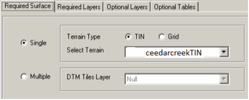
Close the table. We are almost done with GeoRAS pre-processing. The last step is to create a GIS import file for HEC-RAS so that it can import the GIS data to create the geometry file. Before creating an import file, make sure we are exporting the right layers. Click on RAS Geometry-> Layer Setup, and verify the layers in each tab. The required surface tab should have baxter_tin for single Terrain option.
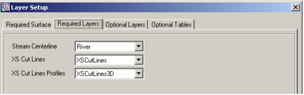
The Required Layers tab should have River, XSCutLines and XSCutLines3D for Stream Centerline, XSCutmLines and XSCut Lines Profiles, respectively.
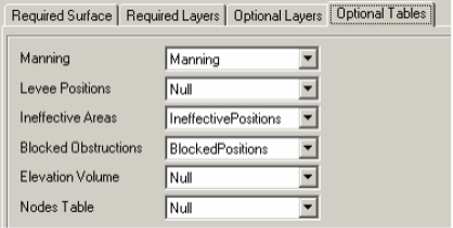
In the Optional Layers tab, make sure the layers that are empty are set to Null.

Finally, verify the tables and Click OK.
After verifying all layers and tables, click on RAS Geometry ->Export GIS Data.
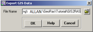
Confirm the location and the name of the export file (GIS2RAS in this case), and click OK. This process will create two files: GIS2RAS.xml and GIS2RAS.RASImport.sdf. Click OK on the series of messages about computing times. You are done exporting the GIS data! The next step is to import these data into a HEC-RAS model. Save the map document. You can either close the ArcMap session or leave it running.
8.12. Importing Geometry data into HEC-RAS
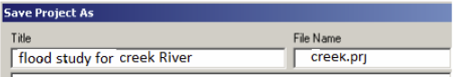
Launch HEC-RAS by clicking on Start->Programs->HEC->HEC-RAS->HEC-RAS 4.0.Save the new project by going to File->Save Project As.. and save as creek.prj in your working folder as shown below: Entering Flow Data and Boundary Conditions
Click OK.
To import the GIS data into HEC-RAS, first go to geometric data editor by clicking on Edit->Geometric Data… In the geometric data editor, click on File->Import Geometry Data->GIS Format. Browse to creekRAS.RASImport.sdf file created in GIS, and click OK. The import process will ask for your inputs to complete. In the Intro tab, confirm US Customary Units for Import data as and click Next.

Confirm the River/Reach data, make sure all import stream lines boxes are checked, and click Next.
Confirm cross-sections data, make sure all Import Data boxes are checked for crosssections, and click OK (accept default values for matching tolerance, round places, etc).
Since we do not have Storage areas, click Finished-Import Data. The data will then be imported to the HEC-RAS geometric editor as shown below:
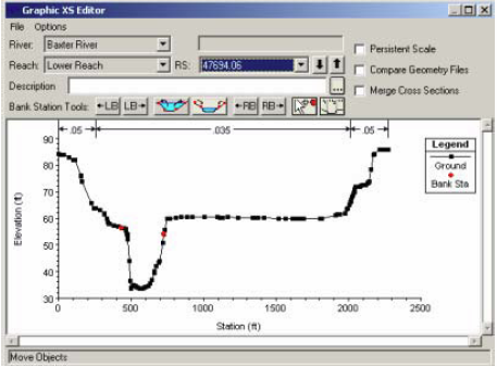
Save the geometry file by clicking File->Save Geometry Data. Before you proceed, it is a good practice to perform a quality check on the data to make sure no erroneous information is imported from GIS. You can use the tools in Geometric editor to perform the quality check. One of the best tools for editing cross-sections in HEC-RAS is the graphical cross-section editor. In the geometric editor, go to Tools->Graphical Crosssection Edit.
You can use the editor to move bank stations, change the distribution of Manning’s number, add/move/delete ground points, edit structure, etc.
A cross-section in HEC-RAS can have up to 500 elevation points. Generally these many points are not required, and also when we extract cross-sections from a terrain using HEC-GeoRAS, we get a lot of redundant points. This issue can be handled by using the cross-section filter in HECRAS. In the Geometric data editor, click on ToolsCross Section Points Filter.
In the Cross Section Point Filter, select the Multiple Locations tab. From the River drop down menu, select (All Rivers) option, and click on the select arrow button to select all cross-sections for all reaches. Then select the Minimize Area Change tab at the bottom, and enter 250 for the number of points to trim cross-sections down to. The minimize area change will reduce the impact of change in cross-sectional area as a result of points removal. Click Filter Points on Selected XS button.

You will get a summary of number of points removed for the filtered cross-sections. You will notice that only a few cross-sections had points removal. Close the summary results box. You can select the Single Location tab to see the effect of points removal on the cross-sections.
Another main task that we want to do is to edit data related to structures. Since we have only one bridge, we will edit its information because details such as deck elevation and number of piers are usually not exported by HEC-GeoRAS. Click on Bridge/Culvert editing button and select the Railroad bridge on the Lower Reach of the Baxter River.
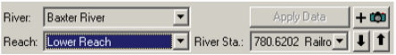
You will see that the deck elevation is not complete. The bridge does not even cross the river in this case! So we will edit this information.
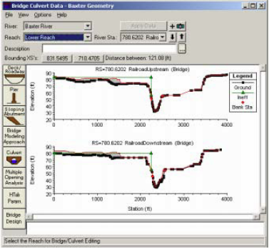
Click on Deck/Roadway editor, and delete all information (you can select the Cells and press Delete on the key board similar to an Excel operation). We will approximate the bridge width to about 1200 ft (station 2200 to 3400), deck elevation as 84 ft (high chord) and 6ft deep (low chord) as shown below:
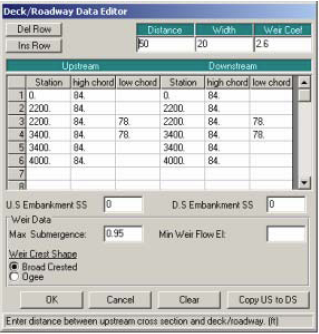
Click on the Copy US to DS button to copy the information from upstream to downstream, and click OK. Next, we will enter pier information. We will assume twelve 10 ft wide piers with a spacing of 100 ft. Click on Bridge Design button , and enter the information as shown below:
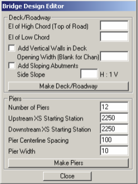
Click on Make Piers, and then click Close. The bridge should now look similar to the figure shown below:
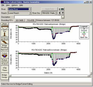
You need to know the actual bridge condition to be able to accurately enter this information, but for this tutorial we have used our intuition (and creativity!) in designing the bridge. After you are done editing the bridge data, close the bridge/culvert editor, save geometry data and close the geometric editor. We are done with geometric data! The next step is to enter flow data. For this tutorial we will run the model in steady state condition.
8.13. Entering Flow data and boundary conditions
Flows are typically defined at the most upstream location of each river/tributary, and at junctions. There are situations where you need to define flows at additional locations, but for this tutorial we will use the typical case. Each flow that needs to be simulated is called a profile in HEC-RAS. For this exercise, we will create three hypothetical profiles. In the main HEC-RAS window, click on Edit->¬Steady Flow Data. Enter 3 for number of profiles, and click Apply Data. Enter hypothetical flow conditions for these profiles as shown below:
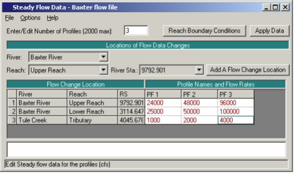
The flow conditions defined in the above window are upstream conditions. To define downstream boundary, click on Reach Boundary Conditions. Then select Downstreamfor Baxter River Lower Reach, click on Normal Depth, and enter 0.001.
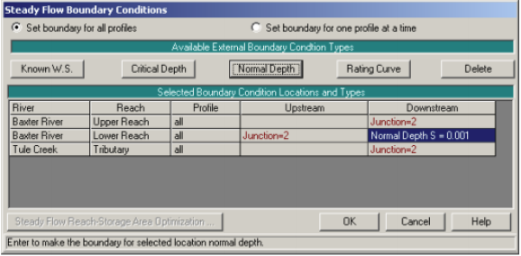
Click OK. Save the flow data (give whatever title you like), and close the Steady Flow editor.Now we are ready to run HEC-RAS!
8.14. Running the model in HEC-RAS
In the main HEC-RAS window, click on Run->Steady Flow Analysis.
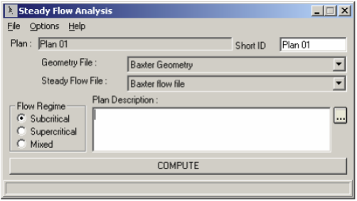
Select the Subcritical Flow Regime, and click on the COMPUTE button. (Note: If you get an error, you will need to modify geometry or flow data based on error messages to run the simulation successfully).
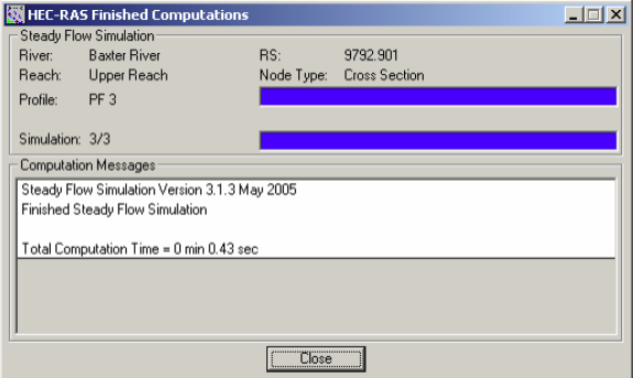
After successful simulation, close the computation window and the steady flow window. We will now export HEC-RAS results to ArcGIS to view the inundation extent, but before this step, you should look at the output results and verify them in HEC-RAS. This will help identify any errors in the input data and fix them, and run the simulation again, if necessary.
8.15. Exporting HEC-RAS outputs
To export the data to ArcGIS click on File-> Export GIS Data in the main HEC-RAS window. Since we ran the model with three profiles, we can choose which profile we would like to export. Click on Select Profiles to Export button, and choose the profile you want to export. For this exercise we will choose the one with maximum flow (PF3), and accept the default export options.
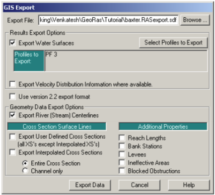
8.16. Flood inundation mapping
In ArcMap (if you closed baxter_georas.mxd earlier, open it) click on Import RAS SDFfile button to convert the SDF file into an XML file. In the Convert RAS Output ASCII File to XML window, browse to Baxter.RASexport.sdf, and click OK. The XML file will be saved with the input file name in the same folder with an xml extension.

Now click on RAS->Mapping -> Layer Setup to open the post processing layer menu as shown below:
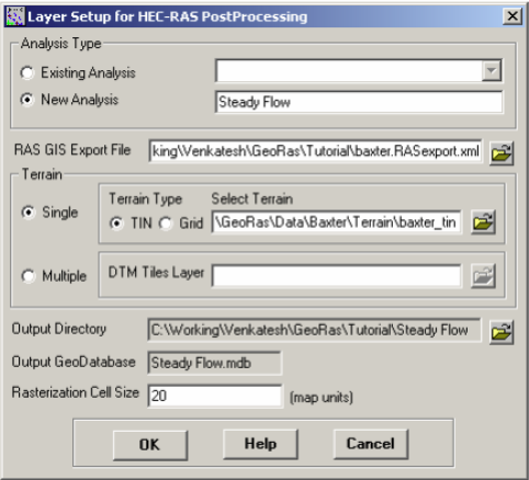
In the layer setup for post-processing, first select the New Analysis option, and name the new analysis as Steady Flow. Browse to Baxter..RASexport.xml for RAS GIS Export File. Select the Single Terrain Type, and browse to baxter_tin. Browse to your working folder for Output Directory. HEC-GeoRAS will create a geodatabase with the analysis name (Steady Flow) in your output directory. Accept the default 20 map units for Rasterization Cell Size. Click OK. A new map (data frame) with the analysis name (Steady Flow) will be added to ArcMap with the terrain data. At this stage the terrain TIN (baxter_tin) is also converted to a digital elevation model (DEM) and saved in the working folder (Steady Flow) as dtmgrid. The cell size of dtmgrid is equal to the Rasterization Cell Size you chose in the layer setup window.
Next click on RAS Mapping->Read RAS GIS Export File. This will create a bounding polygon, which basically defines the analysis extent for inundation mapping, by connecting the endpoints of XS Cut Lines.
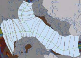
Next click on RAS Mapping->Read RAS GIS Export File. This will create a bounding polygon, which basically defines the analysis extent for inundation mapping, by connecting the endpoints of XS Cut Lines.
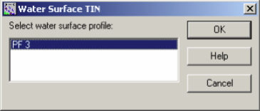
This will create a surface with water surface elevation for the selected profile. The TIN (tP003) that is created in this step will define a zone that will connect the outer points of the bounding polygon, which means the TIN will include area outside the possible inundation.
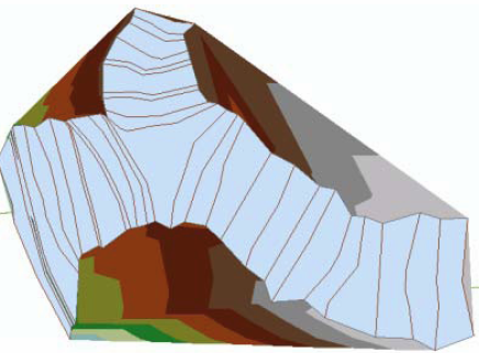
At this point we have a water surface (tP003) TIN, and we have an underlying terrain (baxter_tin and dtmgrid). Now we will subtract the terrain (dtmgrid) from the water surface TIN, by first converting the water surface TIN to a grid. Click on RAS Mapping -> Inundation, Mapping -> Floodplain Delineation. Again, select PF3 (profile with highest flow), and click OK. At this stage the water surface TIN (tP003) is first converted to a GRID, and then dtmgrid is subtracted from the water surface grid. The area with positive results (meaning water surface is higher than the terrain) is flood area, and the area with negative results is dry. All the cells in water surface grid that result in positive values after subtraction are converted to a polygon, which is the final flood inundation polygon.
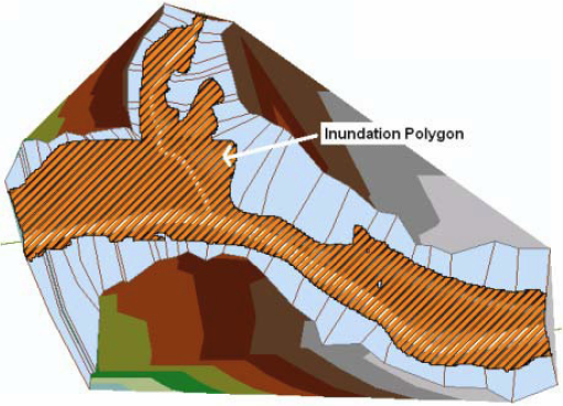
Save the ArcMap document. Congratulations, you have successfully concluded the HECGeoRAS tutorial!