A static Jupyter Notebook for automatic radar-based flood extent mapping is shown below. The notebook can be accessed on GitHub or directly executed in Binder or Google Colab. Please find below the links to the respective platforms: 
![]()
![]()
 The objective of this Recommended Practice is to determine the extent of flooded areas. The usage of Synthetic Aperture Radar (SAR) satellite imagery for flood extent mapping constitutes a viable solution with fast image processing, providing near real-time flood information to relief agencies for supporting humanitarian action. The high data reliability as well as the absence of geographical constraints, such as site accessibility, emphasize the technology’s potential in the field. This Jupyter Notebook covers the full processing chain from data query and download up to the export of a final flood mask product by utilizing open access Sentinel-1 SAR data. The tool's workflow follows the UN-SPIDER Recommended Practice on Radar-based Flood Mapping and is illustrated in the chart below. After entering user specifications, Sentinel-1 data can directly be downloaded from the Copernicus Open Access Hub. Subsequently, the data is processed and stored in a variety of output formats.
  File Structure The Jupyter Notebook file constitutes the directory of origin. Additional data is contained in subfolders. Sentinel-1 images need to be stored in a subfolder called 'input'. If no image is provided, the subfolder will automatically be created when accessing and downloading data from the Copernicus Open Access Hub through this tool. If an area of interest (AOI) file is available (supported formats: GeoJSON, SHP, KML, KMZ), it needs to be placed in a subfolder called 'AOI'. If none are available, an interactive map will allow to manually draw the area of interest. For reasons of automatic file selection, it is recommended to place only one AOI file in the respective folder. However, if multiple files exist, GeoJSON files are prioritized followed by SHP, KML, and KMZ. The processed data is stored in a subfolder called 'output'. In order to run the tool with no user interaction, all inputs must be clearly defined. This means that the 'input' subfolder must include one single Sentinel-1 image and the 'AOI'subfolder one single AOI file. All other scenarios do require manual interaction such as downloading data or defining an AOI. Limitations Difficulties in detecting flooded vegetation and floods in urban areas due to double bounce backscatter. If water and non-water are very unequally distributed in the image, the histogram might not have a clear local minimum, leading to incorrect results in the automatic binarization process. Important The Jupyter Notebook takes advantage of the ESA SNAP API Engineand requires installation of the SNAP-Python interface snappy. Click here for further information. Furthermore, the Jupyter Notebook Extensions Codefolding, ExecuteTime and Table of Contents (2)are used for the most convene performance. ## User Input
  Please specify in the code cell below i) the polarisation to be processed, ii) whether data shall be downloaded from the Copernicus Open Access Hub with respective sensing period and login details, and iii) whether intermediate results should be plotted during the process.
# polarisations to be processed
polarisations = 'VH'                              # 'VH', 'VV', 'both'

# download image from Copernicus Open Access Hub
download = {
    'imageDownload'     : True,                   # 'True', 'False'
    'period_start'      : [2020, 11, 5],          # format: [Year, Month, Day]
    'period_stop'       : [2020, 11, 13],         # format: [Year, Month, Day]
    'username'          : 'username',             # username for login
    'password'          : 'password'              # password for login
}

# show intermediate results if set to 'True'
plotResoluts = True                               # 'True', 'False'
Intialization This section loads relevant Python modules for the following analysis and initializes basic functionalities.
# Click to run
Download Image This section allows interactive data access and download from the Copernicus Open Access Hub. If an AOI file is given in the 'AOI' subfolder, the tool searches and displays available Sentinel-1 images accordingly. If no AOI file is provided, the search bar on the left side of the interactive map can be used to find the desired region. The AOI can be then be selected and manipulated manually by using the drawing tool. Clicking the Search button below the map will load available images. If multiple AOIs are drawn, only the last one is considered. When hovering over a Sentinel-1 image, the tile index and ingestion date are shown. The table below summarizes information on all available tiles and allows the download. The data is stored in the automatically created 'input' subfolder. The Open Access Hub maintains an online archive of at least the latest year of products for immediate download. Access to previous products that are no longer available online will automatically trigger the retrieval from the long term archives. The actual download can be initiated by the user once the data are restored (within 24 hours).
# Click to run
 Loading... Successfully connected to Copernicus Open Access Hub.
  Product 9d5fefa0-7d53-461c-804a-61fb01ce64b5 is online. Starting download. Downloading: 100%|██████████| 991M/991M [00:44<00:00, 22.3MB/s] MD5 checksumming: 100%|██████████| 991M/991M [00:02<00:00, 391MB/s] ## Processing
  If more than one Sentinel-1 image exists in the 'input' subfolder, the user can select which one is to be used for the processing. The subset is generated according to the AOI file in the 'AOI' subfolder. If no AOI file is provided, an interactive map allows drawing the area of interest. Subsequently, the following processing steps are performed:
- Apply Orbit File: The orbit file provides accurate satellite position and velocity information. Based on this information, the orbit state vectors in the abstract metadata of the product are updated. The precise orbit files are available days-to-weeks after the generation of the product. Since this is an optional processing step, the tool will continue the workflow in case the orbit file is not yet available to allow rapid mapping applications.
- Thermal Noise Removal: Thermal noise correction is applied to Sentinel-1 Level-1 GRD products which have not already been corrected.
- Radiometric Calibration: The objective of SAR calibration is to provide imagery in which the pixel values can be directly related to the radar backscatter of the scene. Though uncalibrated SAR imagery is sufficient for qualitative use, calibrated SAR images are essential to the quantitative use of SAR data.
- Speckle Filtering: SAR images have inherent texturing called speckles which degrade the quality of the image and make interpretation of features more difficult. Speckles are caused by random constructive and destructive interference of the de-phased but coherent return waves scattered by the elementary scatter within each resolution cell. Speckle noise reduction can be applied either by spatial filtering or multilook processing. A Lee filter with an X, Y size of 5, 5 is used in this step.
- Terrain Correction: Due to topographical variations of a scene and the tilt of the satellite sensor, distances can be distorted in the SAR images. Data which is not directly directed towards the sensor’s Nadir location will have some distortion. Therefore, terrain corrections are intended to compensate for these distortions to allow a realistic geometric representation in the image.
- Binarization: In order to obtain a binary flood mask, the histogram is analyzed to separate water from non-water pixels. Due to the side-looking geometry of SAR sensors and the comparably smooth surface of water, only a very small proportion of backscatter is reflected back to the sensor leading to comparably low pixel values in the histogram. The threshold used for separation is automatically calculated using scikit-image implementations and a combined use of the minimum method and Otsu's method. The GlobCover layer of the European Space Agency is used to mask out permanent water bodies.
- Speckle Filtering: A Median filter with an X, Y size of 7, 7 is used in this step.
# Click to run
Selected: S1AIWGRDH1SDV20201111T11454820201111T114613035200041C270A8E.zip 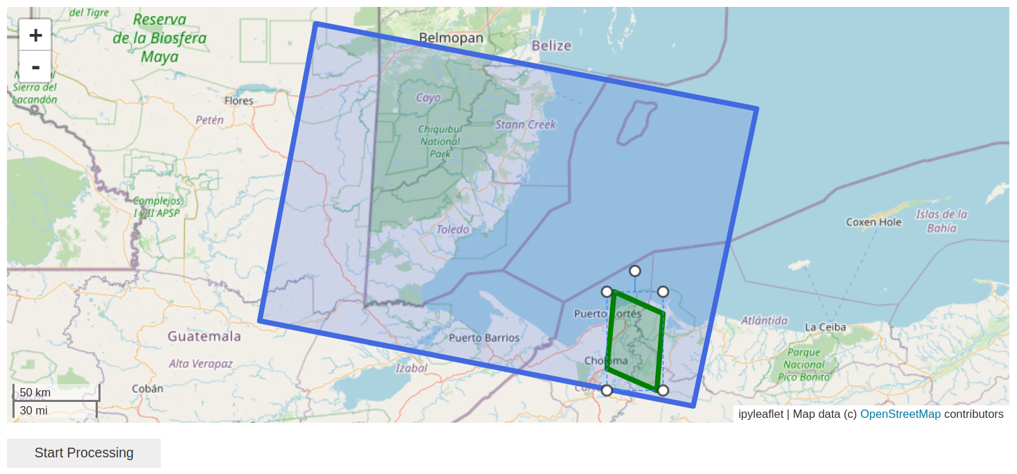 Subset successfully generated. 1. Apply Orbit File: --- 0.02 seconds --- 2. Thermal Noise Removal: --- 0.01 seconds --- 3. Radiometric Calibration: --- 0.03 seconds --- 4. Speckle Filtering: --- 0.01 seconds --- 5. Terrain Correction: --- 0.05 seconds --- 6. Binarization: --- 14.39 seconds --- 7. Speckle Filtering: --- 0.01 seconds --- 8. Plot: --- 55.75 seconds ---
 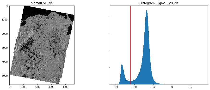 Data Export
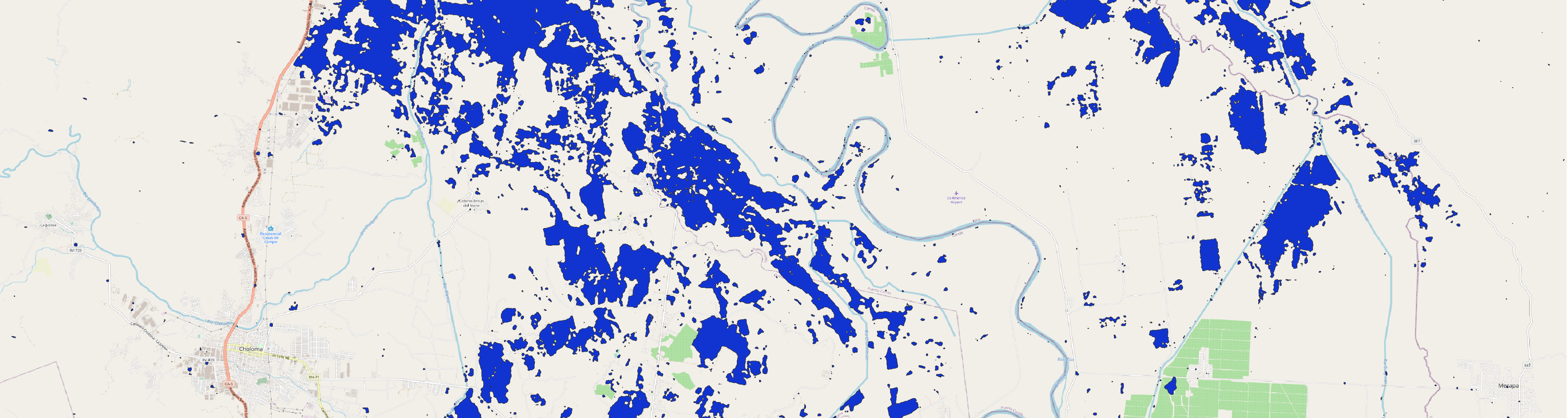
 The processed flood mask is exported as GeoTIFF, SHP, KML, and GeoJSON and stored in the 'output'subfolder. An interactive map shows the flood mask.
# Click to run
Exporting... 1. GeoTIFF: --- 31.88 seconds --- 2. SHP: --- 23.53 seconds --- 3. KML: --- 0.55 seconds --- 4. GeoJSON: --- 1.68 seconds --- Files successfuly stored under /home/eouser/Desktop/Recommended Practices/output. 