Step 1:
- Data preparation
This process must apply to both images.
Unzip the Sentinel-1 data in your working directory, Open SNAP software and call SAR images by clicking on File > Open Product and then selecting the manifest.safe file.
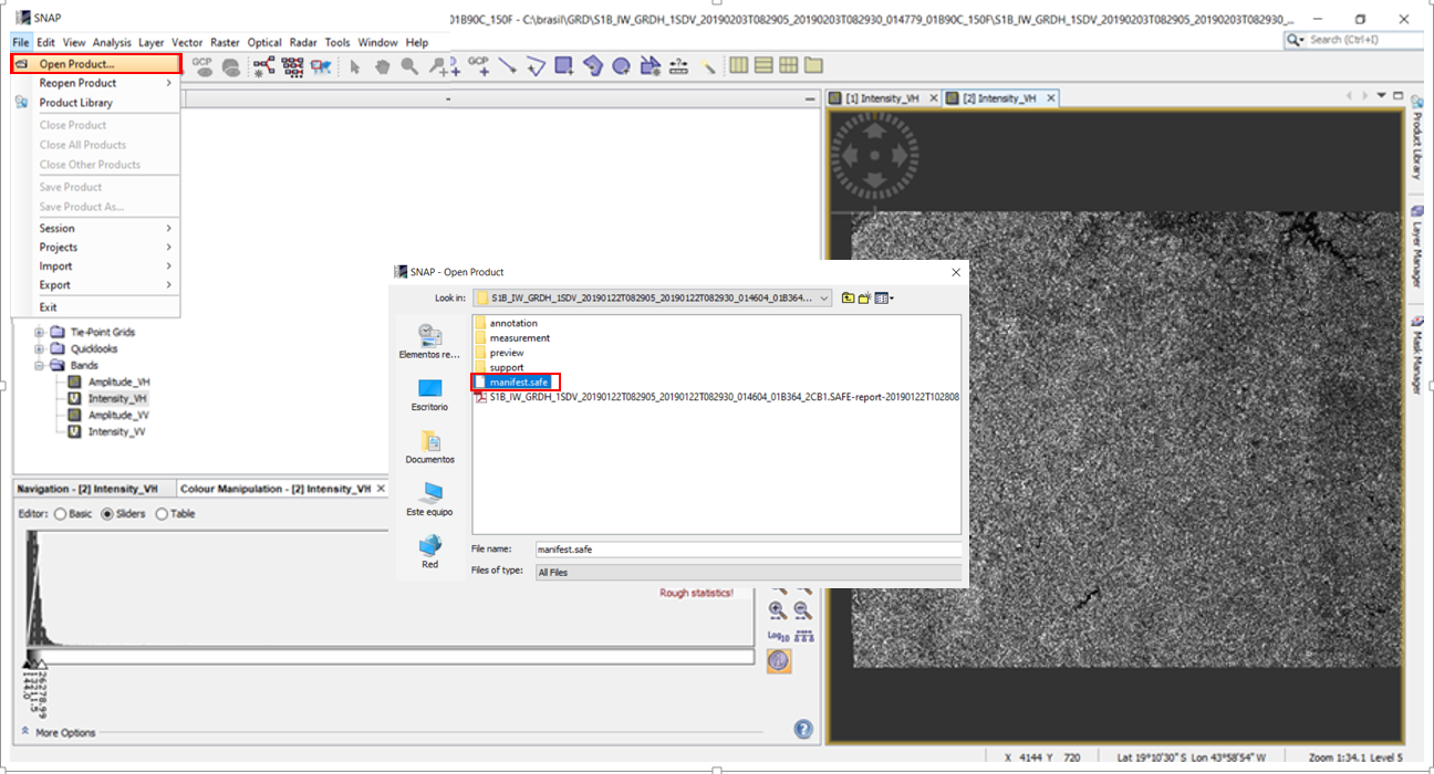
Figure 1
- Apply Orbit File
This process must be applied to both images.
The orbit file provides an accurate position of SAR image and the update of the original metadata of SAR product, the orbit file is automatically downloaded from SNAP software. For this recommended practice, the "apply orbit file" procedure can be optional; nevertheless, it's highly recommended to ensure a successful spatial coregistration process.
Select Radar > Apply Orbit File, and then define all parameters according to Figure 2.
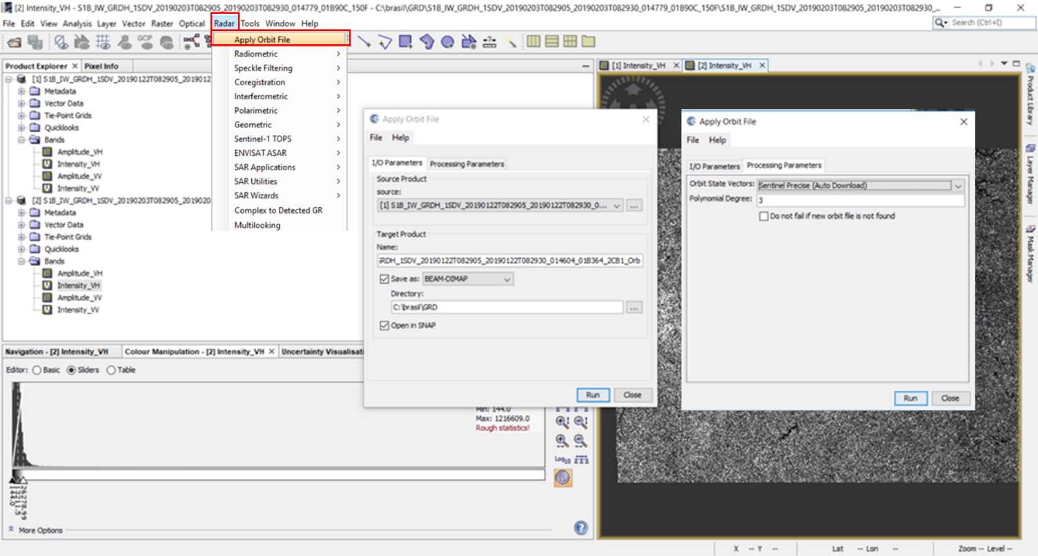
Figure 2
- Calibration
Select Radar > Radiometric > Calibrate, and set the “Processing Parameters”, select all polarizations and select Sigma0 as output band.
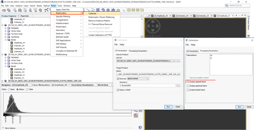
Figure 3
This process must be applied for both images.
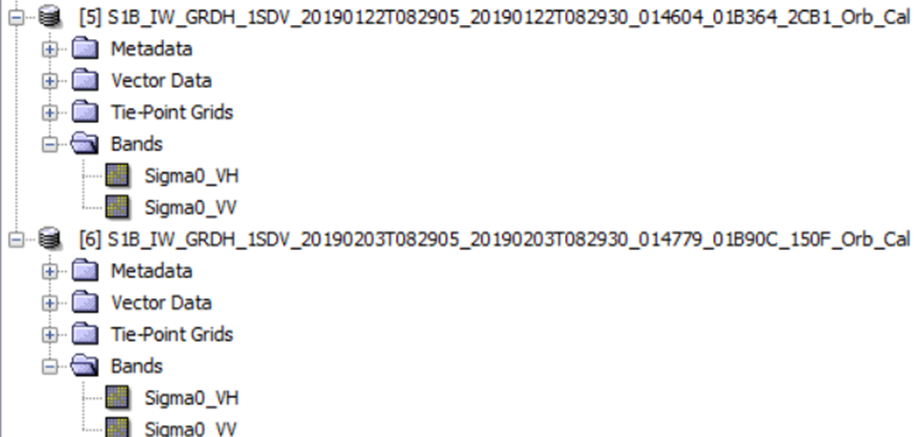
Figure 4
- Speckle Filtering
Select Radar > Speckle Filtering > Single Product Speckle Filter, and set the “Processing Parameters” as shown in Figure 5.
You can select another type of filter according with your expertise; however, we recommend using Lee and Frost filters as they are less degrading to the SAR image.
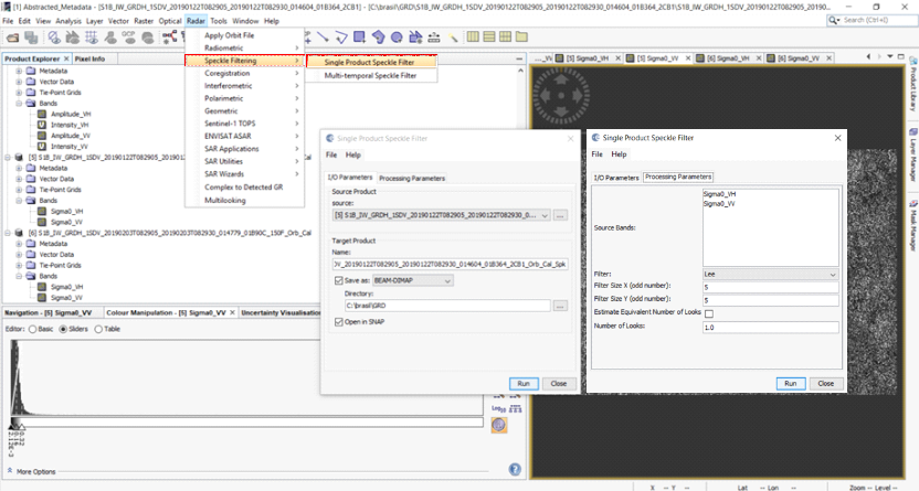
Figure 5
This process must be applied for both images.
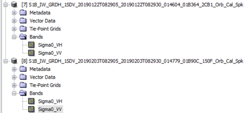
Figure 6
- Geocoding
Click on Radar > Geometric > Terrain Correction > Range-Doppler Terrain Correction, and define all “Processing Parameters” according to Figure 7.
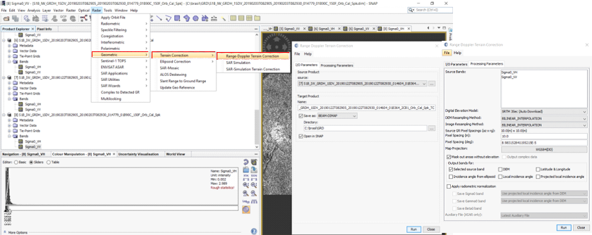
Figure 7
This processs must be applied for both image.
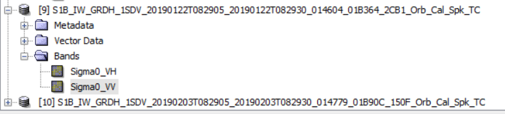
Figure 8
- Subset
To get the same spatial subset to both images, click on View and select the following menu options: Statusbar, Synchronise Image Cursors and Synchronise Image Views.
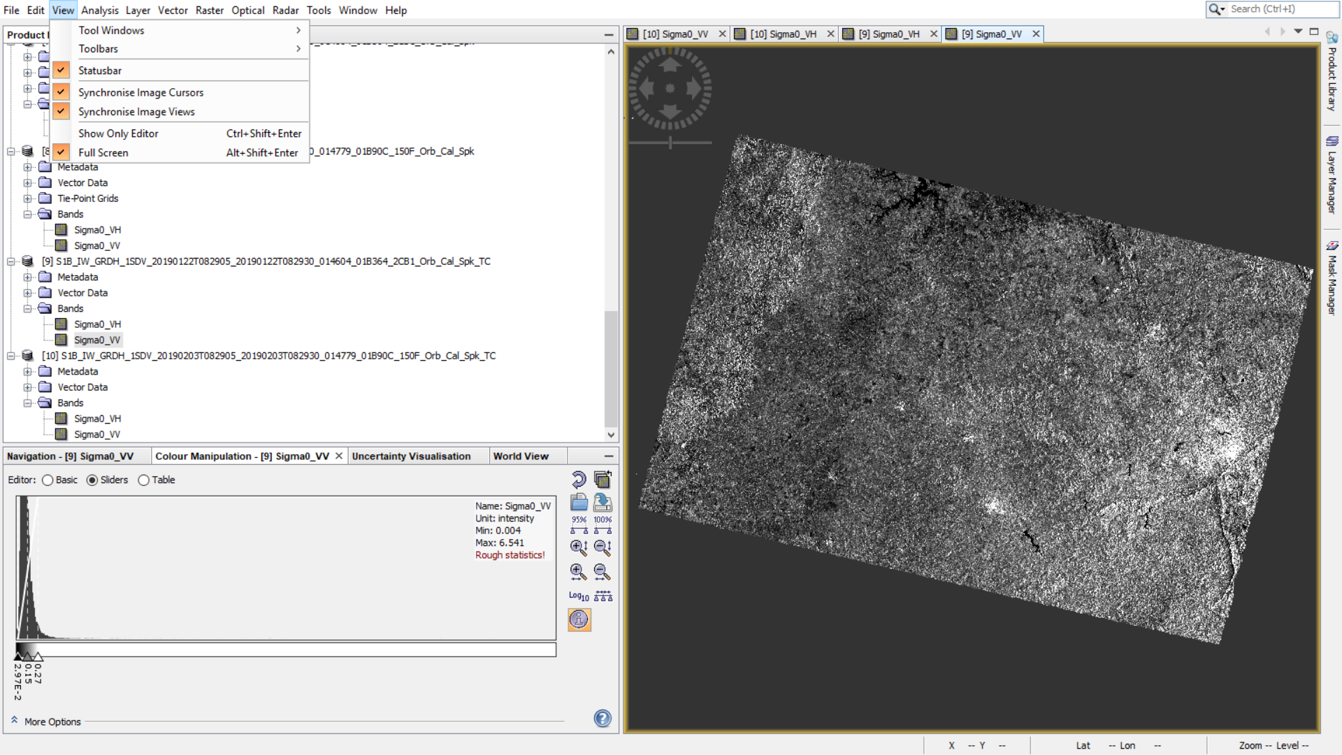
Figure 9
Go to Raster > Subset, specify the area and parameters of the region of interest as shown in Figure 9.
This process must be applied to both images.
To ensure the same spatial coverage for both images, double click on any of the bands (vv or hv) of the second image and start again the “subset processing” as mention above.
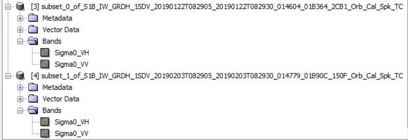
Figure 10
Now, the new subset products must be converted to BEAM-DIMAP format. For this, right click over the name of each new subset product and select Save Product As, rename it if desired, click ok.
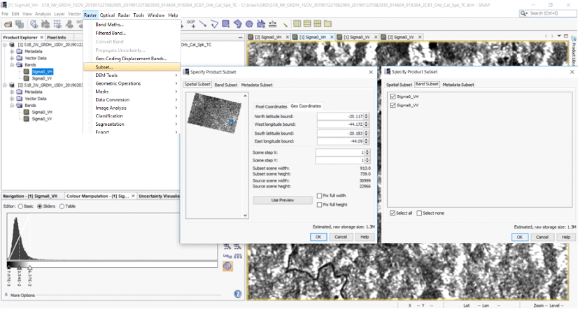
Figure 11
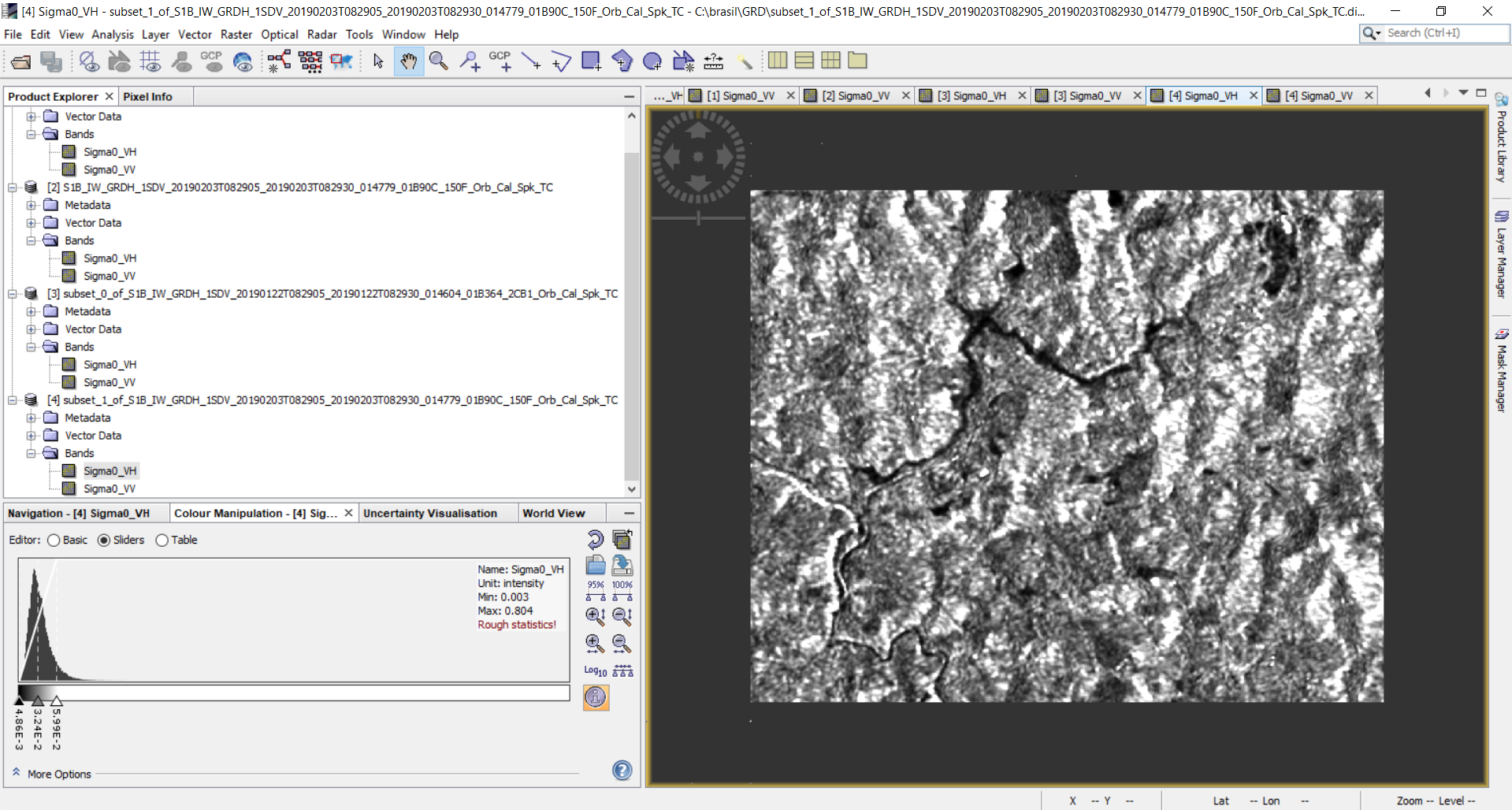
Figure 12
- Corregistration stack
To generate a composite image from SAR data before and after the massive mudslide, a spatial coregistration procedure is necessary. For this, go to Radar > Corresgistration Stack > Tools > Create Stack, click the plus icon and select only the new subset products.
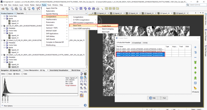
Figure 13
Define the rest of parameters as shown in Figure 14.
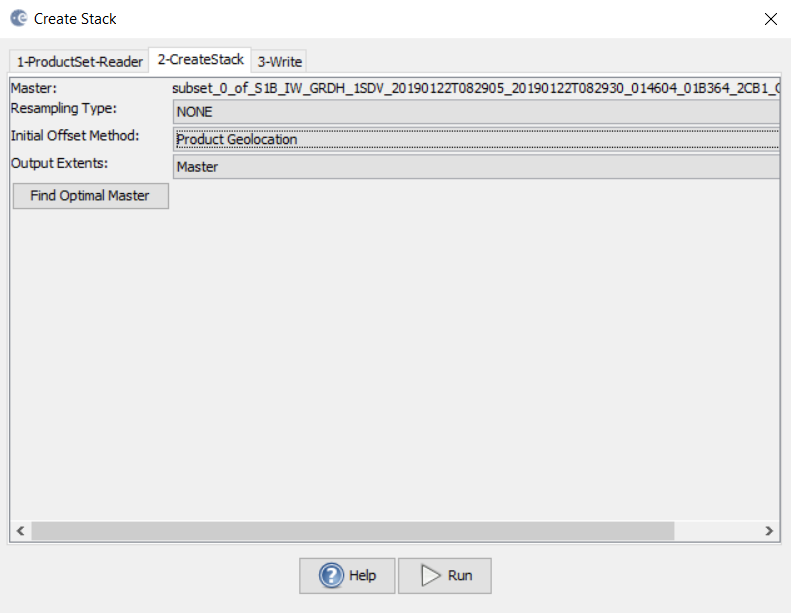
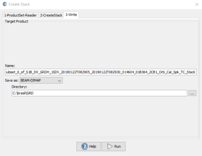
Figure 14
Open the new product as a composite image using the different polarizations. For this, right-click the name of the new product and select Open RGB Image Windows; choose the desired bands.
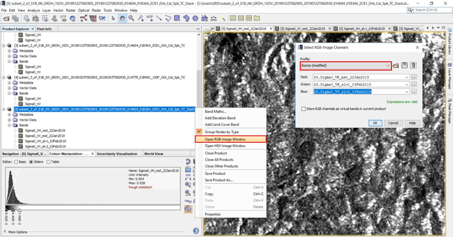
Figure 15
Example of the RGB image composite
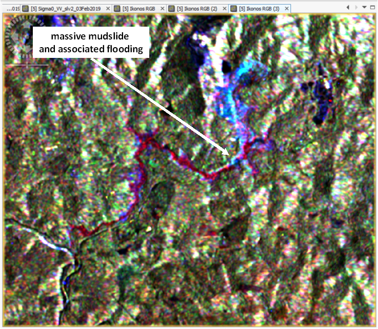
Figure 16
Step 2: Processing
- Change Detection
The Log Ratio is an algorithm used to the change detection procedure using mean ratio operator between two images of the same coverage area but taken at different times. To apply this procedure, click on Radar > SAR Applications > Change Detection, and define the processing parameters according to figure 17.
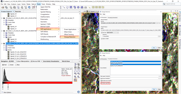
Figure 17
This procedure must be applied for all possible combinations between SAR images before and after the massive mudslide event. The following Log Ratio date combinations are required:
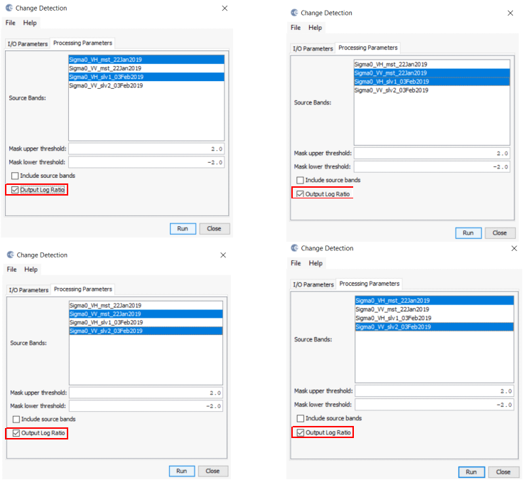
Figure 18
The massive mudslide and flooding area are identified by high-intensity pixels, identification is also possible by very low-intensity pixels. For this reason, PCA is used to regroup the pixel set optimally in order to achieve a digital enhancement of magnitude values associated with the affected area.
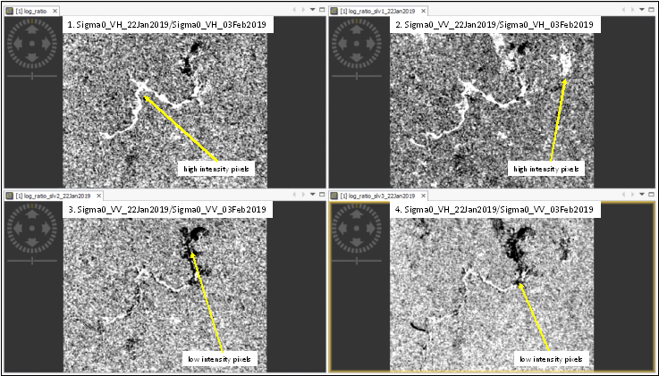
Figure 19
- Coregistration stack (Log Ratio results)
To apply principal components analysis, a composite image from all Log Ratio results must be generated. For this, go to Radar > Corresgistration Stack > Tools > Create Stack, click on plus icon and select the four Log Ratio images. It is important to keep the order of the image combinations as listed in the previous step, "change detection" (Log Ratio):
-
Sigma0_VH_22Jan2019/Sigma0_VH_03Feb2019
-
Sigma0_VV_22Jan2019/Sigma0_VH_03Feb2019
-
Sigma0_VV_22Jan2019/Sigma0_VV_03Feb2019
-
Sigma0_VH_22Jan2019/Sigma0_VV_03Feb2019
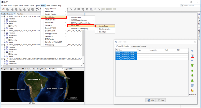
Figure 20
Define the processing parameters according to Figure 21. Rename the file if desired.
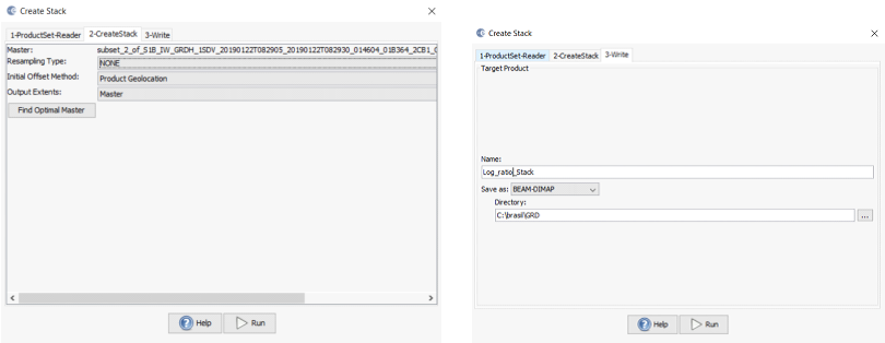
Figure 21
- Apply Principal Components Analysis (PCA)
Click on Raster > Image Analysis > Principal Components Analysis, and call the new product (Log Ratio stack), and select the four Log Ratio images. Define all “Processing Parameters” according to Figure 22.
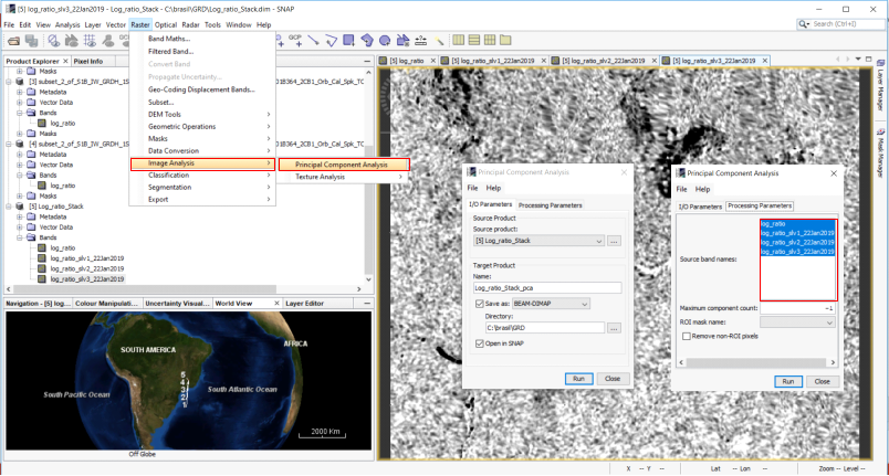
Figure 22
The new product is created by four "out band components" and one "response band". As mention before, PCA implies a new data regrouping (a reversible orthogonal transformation), where towards the first "out band components" the variance is maximized. This means that the more significant pixel information is kept; while towards the last "out band component," all noise or redundant information is separated. The first three components can be used for the next steps. The “response band” represents each basis vector of the “out band components”, high values correspond to a better fit of data; so, this band can be used for the next steps as well.
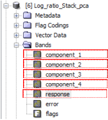
Figure 23
“Out Band Components” results:
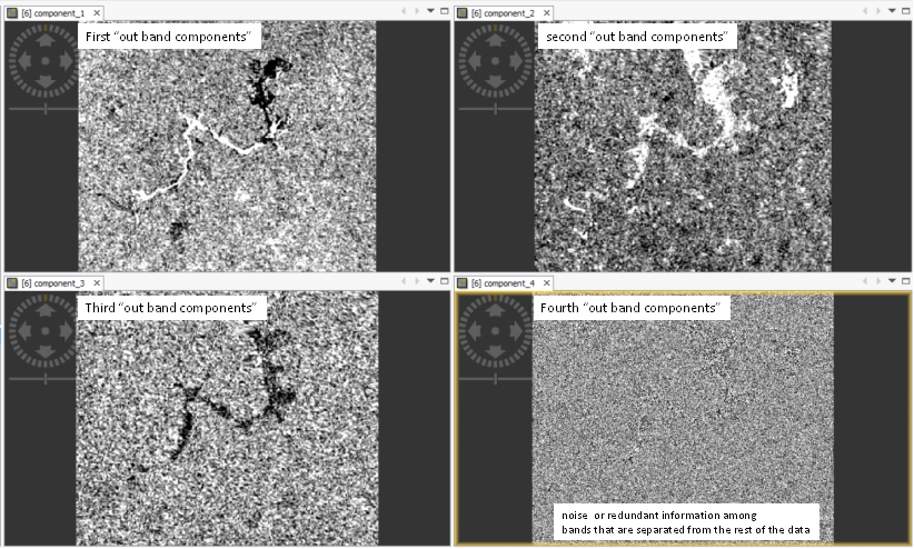
Figure 24
“Response band” result:
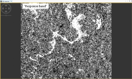
Figure 25
- Supervise image classification
Each of the four final bands contains digital enhancement information about massive mudslide event and associated flooding. The differences in the spatial information provided by the final bands are linked to soil moisture conditions, differences between water bodies or by the large volume of sediments transported during a flood.
Thus the next step is to extract the affected area using a classification procedure. First, it is necessary to define the training polygons. Only two classes were defined: “no mudflow area” and “mudflow”; we recommend visualizing each of the final bands separately.
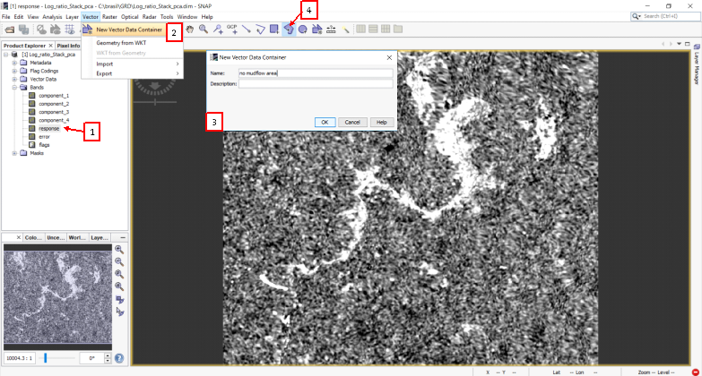
Figure 26
-
double click on the final band selected
-
go to New Vector Data Container and a new window will be opened
-
name the polygon class "no mudflow area" and you can start to draw the polygon contouring
-
if you desired to add another polygon of the same class "no Mudflow area", click on Polygon Drawing Tool and then start to draw it
Figure 26
-
to add a new polygon class, go to New Vector Data Container and a new window will be opened
-
name the new polygon class "mudflow" and click ok
-
click over the image and a new window will open, the two clases are listed, select "mudflow"; now draw the polygon contouring
-
if another polygon of the "now Mudflow area" class is needed, click on Polygon Drawing Tool and start drawing it
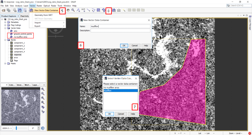
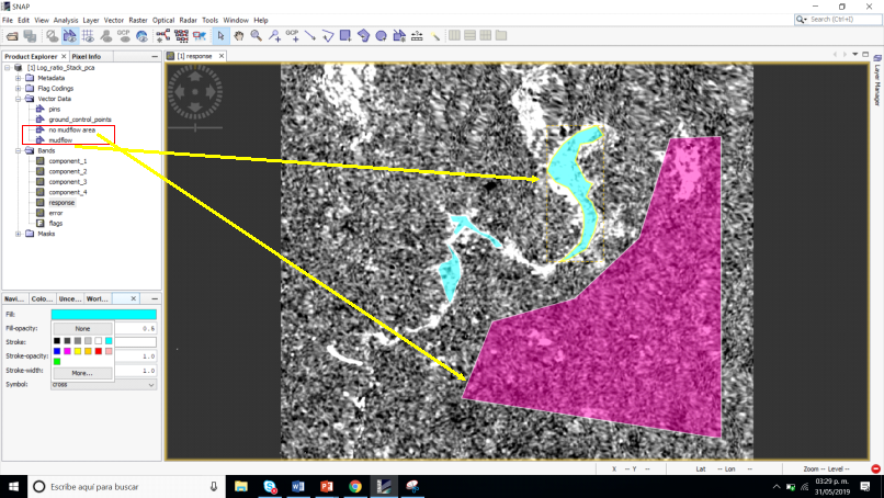
Figure 27
Go to Raster > Classification > Supervised Classification > Maximum Likelihood Classifier
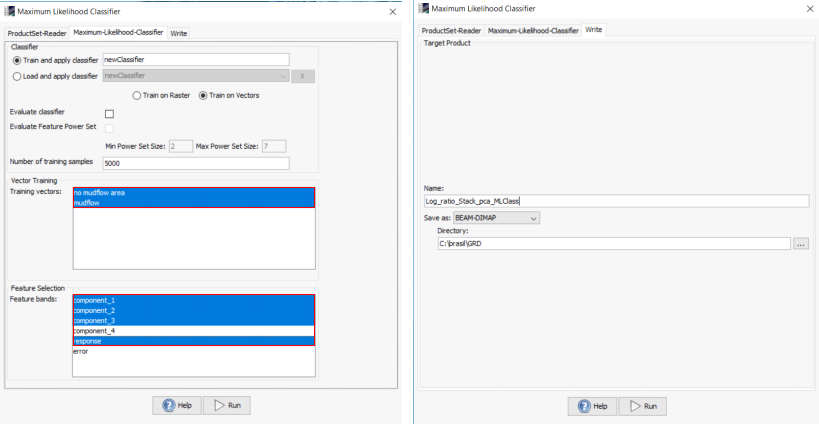
Figure 28
Select the two “training vector” classes previously defined and the “feature bands” (out band components and response band) as shown in the Figure 29.
Supervised classification result:
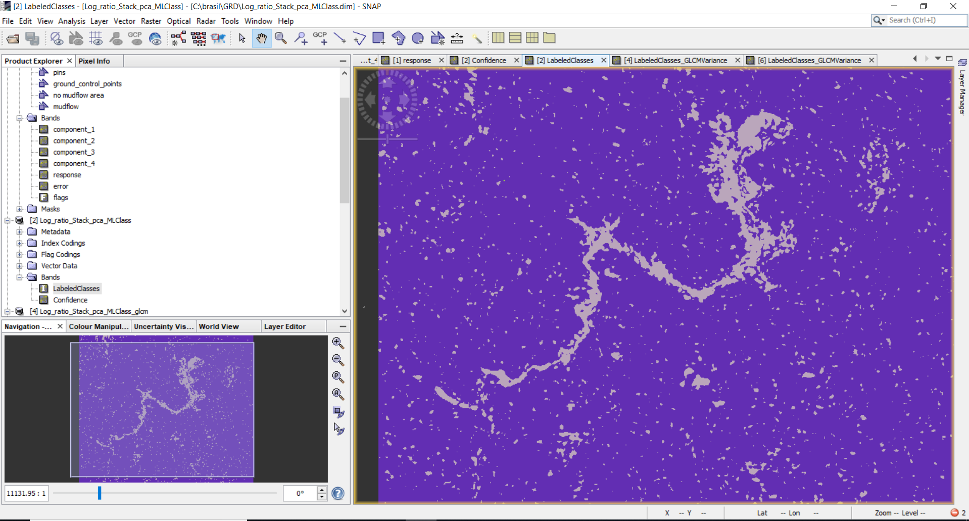
Figure 30
- Apply smooth filtering
To smooth the classified image result and regroup the pixels in an optimal way, a filtering process is needed. For this, go to Raster > Image Analysis > Texture Analysis > Grey Level Co-ocurrence Matrix, select only GLCM Variance option. Define all “Processing Parameters” according to Figure 31 and Figure 32.
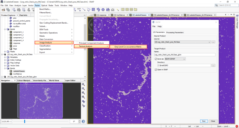
Figure 31
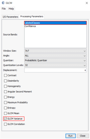
Figure 32
Smooth filtering result:
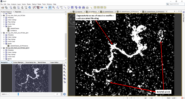
Figure 33
Step 3: Post Processing
- Getting a binary final image
After the smooth filtering procedure, the values of the final classified image convert from binary values to continuous raster cell values (stretch values); thus, converting a raster file to shape format can be complicated. An easy way to get a final binary image again is to apply a Supervised Classification a second time. For this, the last product from the “smooth filtering” procedure must be used to apply the Supervised Classification a second time.
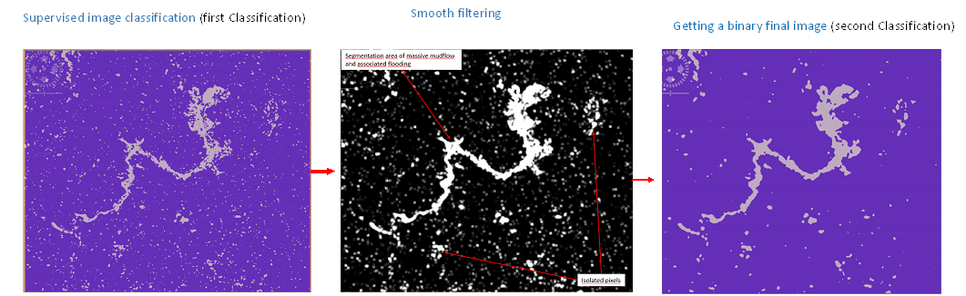
Figure 34
- Convert raster to shape file
Go to File > Export > GeoTIFF and select the last product (Supervised Classification a second time).
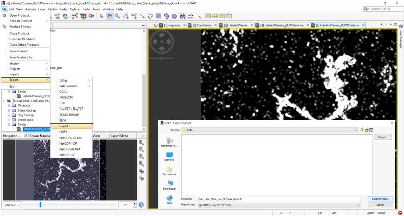
Figure 35
Open QGIS software and click on Raster > Conversion > Poligonize, and call the GeoTiff file.
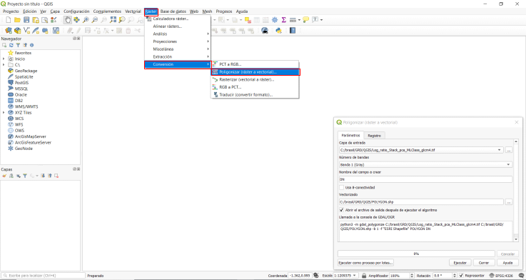
Figure 36
The shape file is generated.
- click the polygon that represents the spatial distribution of the massive mudslide; the polygone will change colour
- go to the layers menu and right-click on the name of the polygone file and go to Export > Save As > Selected Features, save the new shape file as Esri Format

Figure 37
- Visualization of results
Open Snap Software and call the RGB composite image generated in the procedure “Corregistration stack” (Step 1).
Go to File > Import > Vector Data, and call the new shape file as Esri Format. Thus, you can overlap the shape file associated to the affected flooding area with respect to the original SAR data.
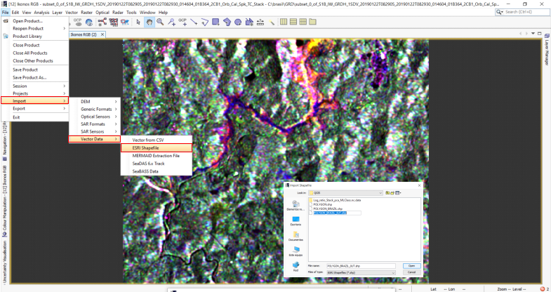
Figure 38
 .
.
GIF 1
The result of this recommended practice was compared with previous information provided by the International Charter Space and Major Disasters, where the massive mudslide was mapped using RapidEye high resolution data acquired after the event.
It is important to mention that the optical satellite image (RapidEye) used to identify the affected area has a higher spatial resolution than Sentinel-1. Despite this, the final results are very similar in spatial terms. This speaks about the effectiveness of our method of mapping this type of disaster event using Sentinel-1.
GIF 2
.png)
.png)
.png)
Figure 39