1. HEC-RAS 2D Model
HEC-RAS 2D flood model was developed by US Army Corp of Engineer’s Hydrological Engineering Center (HEC). The model can solve 1D and 2D flood hazard problems through 1D, 2D and 1D/2D coupling approaches. HEC-RAS 2D model Graphical User Interface (GUI) is shown in Figure-1.

2. HEC-RAS Geometric data
HEC-RAS 2D requires following geometric datasets:
- Digital Elevation Model (DEM)
- Landcover/Landuse Map
- Manning’s n layer
- 2D flow area
- Boundary condition lines
- River cross-sections (in case of 1D and 1D/2D coupling approach)
- Embankments
- Restricted areas (if any)
2.1. Digital Elevation Model
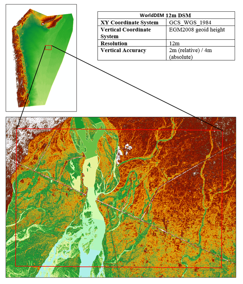
Digital Elevation Model (DEM) represents floodplain terrain in flood model. Globally freely available DEMs (SRTM, ALOS World3D and ASTER) and locally available high resolution can be used for the terrain representation in flood model. In this practice, the 12m WorldDEM DSM provided by Airbus Space and Defense through UN-SPIDER Bonn Office (Figure-2) was used to model topography.
2.2. Manning’s n layer
Manning’s n layer is required to account for infiltration component of water channel, floodplain and its surrounding landcover/landuse types in flood model and can be prepared using the existing landcover data and Manning’s n Table (Chow 1959).
2.3. 2D flow area
2D Flow Area tool is used to determine the flood model computation boundary based on the terrain. Moreover, 2D Flow Area should follow the terrain and cover the minimum area considered for the simulation run in order to optimize the flood model computation time.
2.4. Boundary condition lines
Boundary Condition lines are the cross-sections at upstream and downstream where discharge data in the form of hydrographs (flow or stage) can be provided to the flood model.
3. Hydrological data
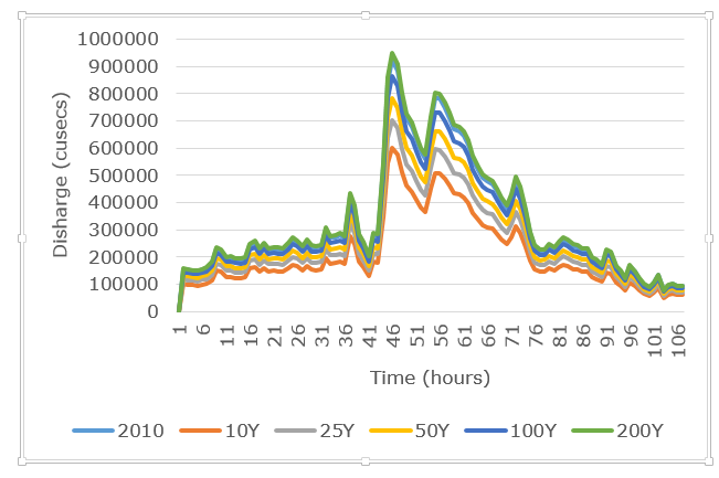
Hydrological data including known event hydrograph and stage height at the upstream and downstream gauge stations are required for model setup, calibration and validation. Designed hydrographs are prepared based on known flood event hydrograph and flood return periods. Moreover, flood return periods can be calculated using flood frequency analysis techniques. In this case study, Flood2010 observed flow hydrograph were used for the calculation of designed hydrographs in addition to the return period calculated through Log Pearson Type III. The following equations were used to calculate factor for designed hydrographs preparation:
Factor = Flood2010 Observed Discharge (Peak) / Flood Return Period Discharge (max)
Designed Hydrograph = Factor * Flood 2010 Observed Hydrograph
Designed hydrograph prepared for the study area are shown in the Figure-3.
4. Satellite imagery / flood maps
Satellite imagery (optical or SAR) and flood maps (hard or soft) of known events are required for the model calibration and validation.
- Download HEC-RAS 2D model from Hydrological Engineering Center (https://earthexplorer.usgs.gov) and install
- Run HEC-RAS 5.0.4
- Create new project [File>New Project]
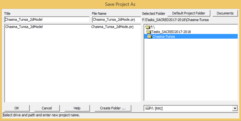
- Write down Project Name and select desired directory as shown in Figure-4
- Finally, save your project
- HEC-RAS uses US Customary Units by default and can be changed to ‘SI Units’ whenever required
- Open RAS Mapper [GIS Tools > RAS Mapper]
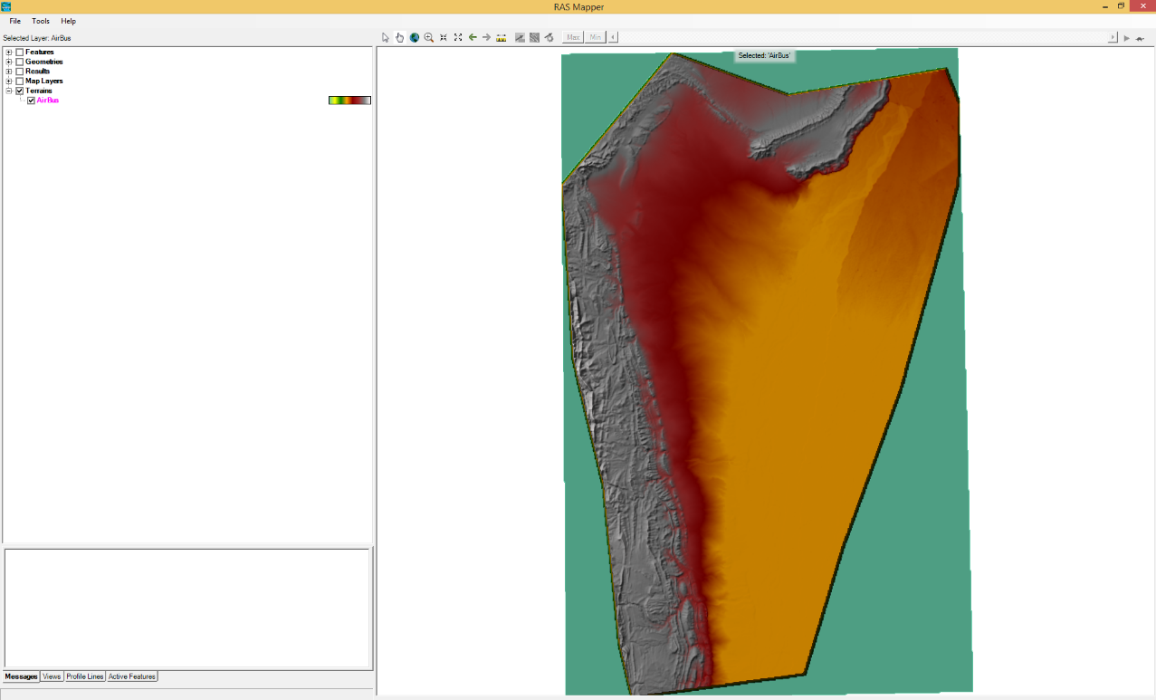
- Right Click on Terrain in the table of contents and click Create New RAS Terrain. Click ‘No’ to define the Project Spatial Reference System (SRS) later in the popup window. Add WorldDEM DSM Layer from desired directory and click ‘Yes’ to use DEM projection as SRS of the project. Created terrain is shown in the Figure-5.
- Double click on Terrain to see terrain properties. Terrain Properties like ‘Z’ Factor can be changed for better visualization of WorldDEM DSM as well as for the determination of the 2D flow area and Boundary condition lines.
- Now right click on Map Layers and select ‘Add New Manning’s n Layer. Following window will popup (Figure-6).
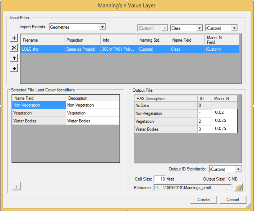
- Add landcover layer from desired directory and define Manning’s n for each class using Manning’s n table (Appendix-I) and click "Create". Created Manning’s n layer is shown following Figure-7.
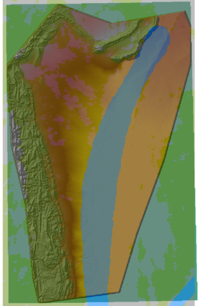
- Save data in RAS Mapper [File > Save] and exit.
- Now open Geometric Data Window from HEC-RAS main GUI [Edit > Geometric Data]
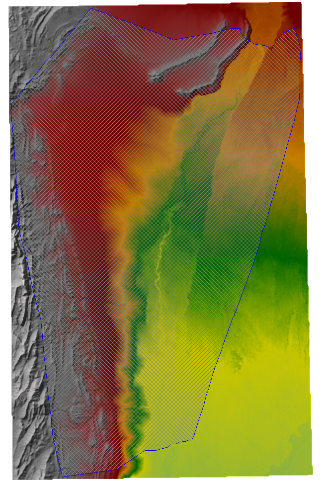
- Select 2D Flow Area and draw/digitize the polygon on the terrain. It may be noted that 2D flow area is drawn based on the historical maximum observed flood limits. Alternatively, 2D flow area can be mapped up to the high altitude land/features. Created 2D Flow Area polygon (in blue) can be seen in the following Figure-8.
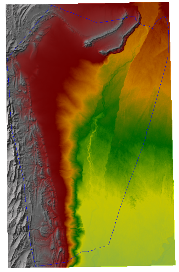
- Click on the 2D Flow Area polygon and select ‘Edit 2D Flow Area’ from right click options. Popup will display as shown in Figure-9
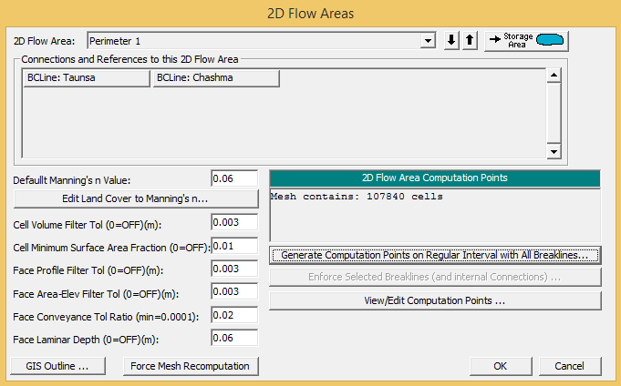
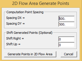
- Click on "Generate Computational Points …" option and provide for DX and DY cell values (shows floodplain grid spacing). Then click on ‘Generate Points in 2D Flow Area’ (Figure-10). Finally, click ‘Ok’ to generate the computation mesh.
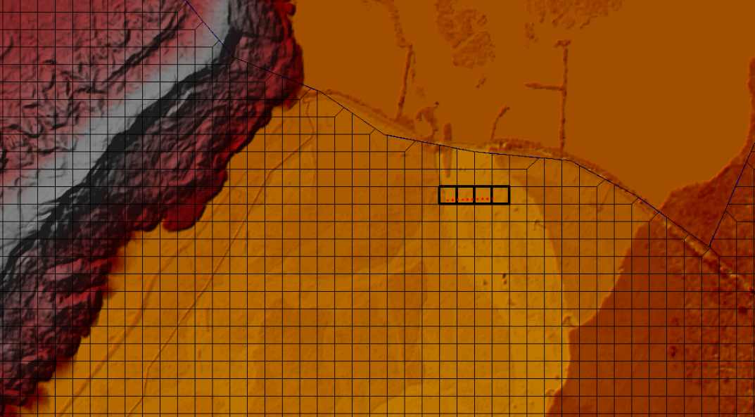
- Computed floodplain mesh can be seen in the flowing Figure-11.
- In order to create 2D Area BC Lines click on. Draw an arc at the gauge station locations i.e. Chashma Barrage D/S station and Taunsa Barrage U/S station where boundary conditions will be applied. Created BC line at the upstream location can be seen in the following Figure-12.
- Save the Geometric Data and exit.
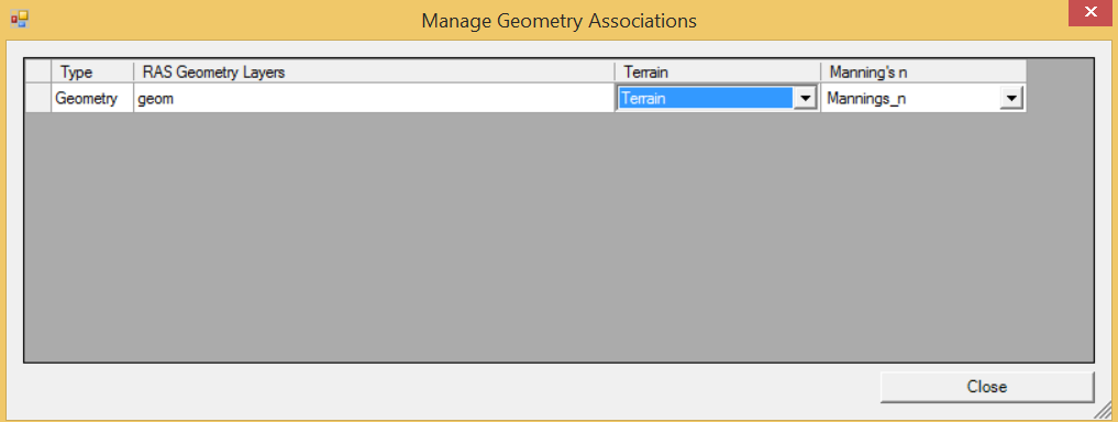
- Now open RAS Mapper and right click on Terrains and Click Manage Terrain Association. Confirm that Terrain and Manning’s n layer are associated with geometry. If not so then select appropriate terrain and Manning’s n layer from dropdown menus and close the window (Figure-13).
- Save RAS Mapper and exit.
- Open Unsteady Flow Data [Edit > Unsteady Flow Data]
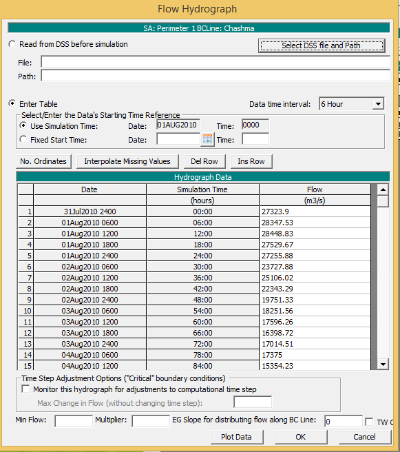
- Click on the ‘BCLine: Chashma_Barrage’ and select ‘Flow Hydrograph’ as Boundary Condition. Select data interval time to 6 Hour or according to the discharge data in your study area. Populate the Hydrograph Data i.e. Flood2010 in our case and EG Slope (bed slope) value as shown in the Figure-14.
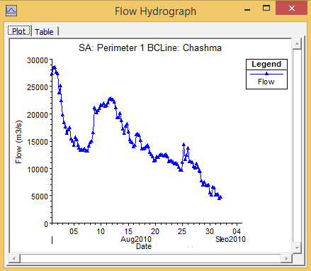
- Click on Plot Data to check the Flow Hydrograph shape. Flow hydrograph of the input data at the upstream boundary condition line is shown below in Figure-15.
- Click Ok to close the Flow Hydrograph window.
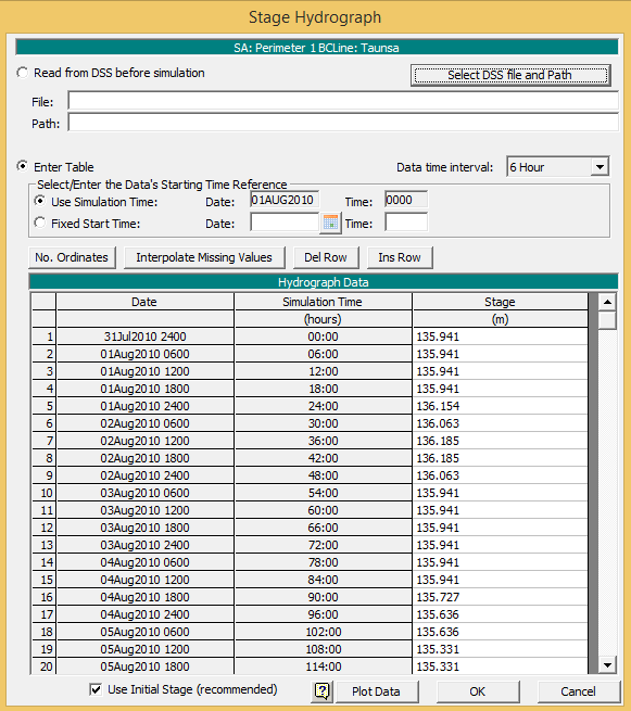
- Likewise, click on ‘BCLine: Taunsa_Barrage’ and select ‘Stage Hydrograph’ as Boundary Condition and insert stage values at the downstream gauge station as shown in Figure-16.
- Save the unsteady flow data [File > Save Unsteady Flow Data As] and close the window.
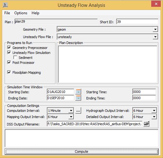
- Now open Unsteady Flow Analysis [Run > Unsteady Flow Analysis]. Select the simulation starting and Ending date and time as per the hydrograph. Computational setting can be made as shown in the Unsteady Flow Analysis window. Smallest the interval, more computation time will be taken by HEC-RAS.
- Check Programs to run and Click Compute. Example of the parameters define in Unsteady Flow Analysis are shown below (Figure-17). Computation will take some time (up to few hours) depending on the computation grid size and output intervals selected.
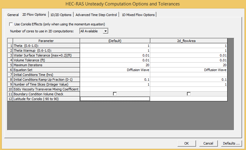
- Diffusive Wave equation [Option>Unsteady Computation Options and Tolerances] was selected for model simulation (Figure-18). Keeping in the flood flow behavior (mixed flow) in your study area you may need to choose Momentum Equation for flood model simulation.
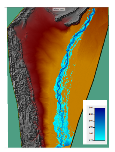
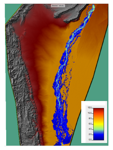
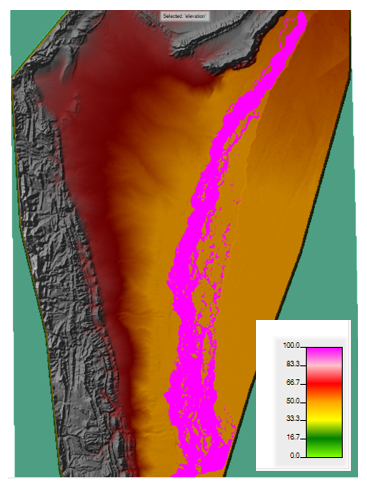
- Simulation results can be viewed in RAS Mapper Window. Flood model main outputs include Depth, Velocity and WSE. Flood model simulated depth, velocity and WSE for known Flood2010 event is shown below (Figure 19-21).
- Simulated flow hydrograph and stage at U/S and D/S stations can be viewed and analyzed [View>Stage and Flow Hydrographs]
- In order to store flood depth, velocity and WSE maps open Manage Result Maps [Tools>Manage Result Maps] in RAS-Mapper window. Then click on ‘Edit Map’ in front of Depth Layer and select ‘Raster based on Terrain’ option and Click ‘Save Map’. Similarly, follow the above mentioned step for velocity and WSE layers. Finally, click on ‘Compute/Update Stored Maps’ to save required layers in directory as Geotiff. Stored maps of the calibrated and validated model output can be then used for the flood hazard maps and flood exposure analysis in GIS environment.
Model calibration
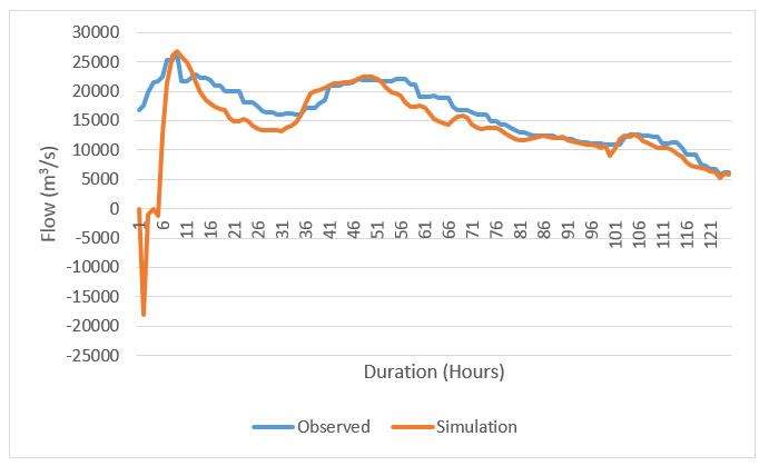
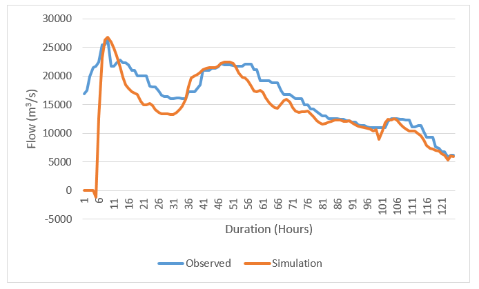
Flood model often do not give satisfactory results in the first run. Hence, flood model has to be calibrated for the desired results. Model Calibration can be has been carried out by adjusting Manning’s n values for main channel and 2D flow area. Manning’s n values plays an important role in model calibration and can be adjusted according their Min, and Max ranges available in the standard hydrological table (Chow, 1959). It may noted here that Manning’s n layers has to be updated whenever there is change in Manning’s n value for any landcover class. Calibration process may requires a number of simulations until observed and simulated discharge and stage height are nearly matched. Following (Figure 22-23) shows simulated and observed hydrograph of the un-calibrated and calibrated flood model at the downstream gauge station.
Model validation
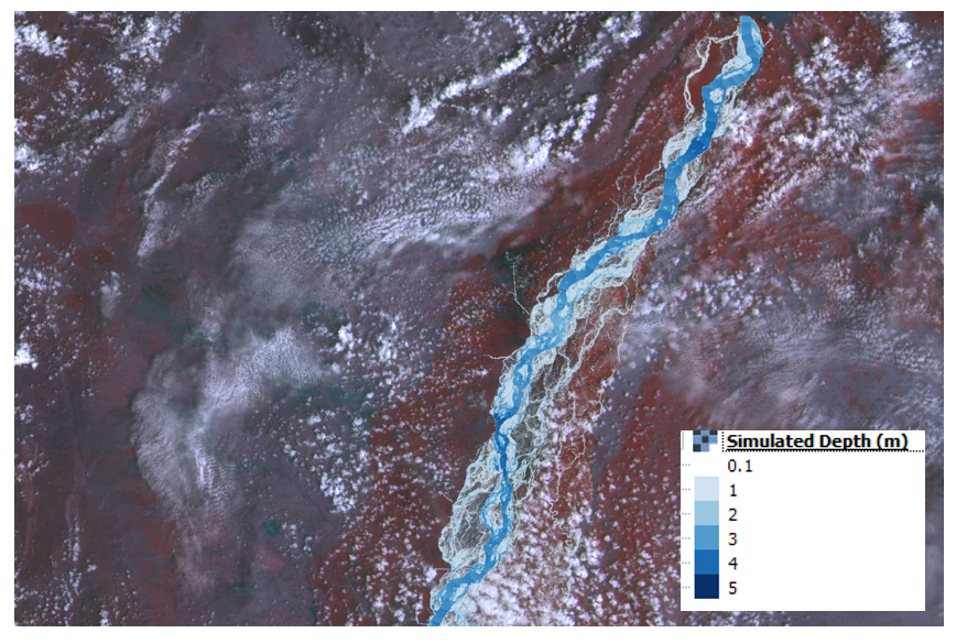
Flood model simulated inundation extent was validated with satellite based observed flood extent. In our case we have compared model results with the Landsat imagery acquired during Flood2010 event. However, cloud free imagery was acquired a week later than peak flood in the study area shown in Figure-24.
Probabilistic flood simulations
Finally, calibrated model was then simulated for the design flood events pertaining to the 2, 5, 10, 25, 50, and 100 years return periods. Kindly repeat Step by Step from Para 23 to 31 for the simulation of the design flood events.
Flood hazard maps
- Load model simulated depth stored maps (Geotiff) [ output of the Step 31] in GIS environment (QGIS or ArcMap)
- Classify the layer based on depth values as per the criteria mentioned in Table-1.
| Depth range | Class |
| < 1m | 1 (very low) |
| 1-2m | 2 (low) |
| 2-3m | 3 (medium) |
| 3-4m | 4 (high) |
| >4m | 5 (very high) |
- Convert/Vectorize raster to polygons and then dissolve output shapefile based on class values.
- Load Landcover dataset of the study area in QGIS or ArcMap.
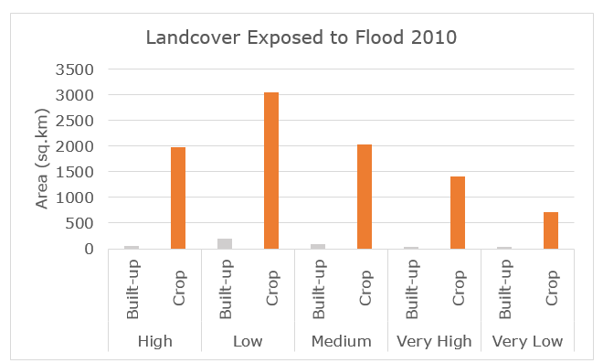
- For landcover exposure to the simulated flood depth and extent, ‘Intersect’ flood depth layer (vector format) with the landcover layer. Then summarize the exposed landcover in the form of graphs/maps. Following graph (Figure-25) shows landcover exposure to the Flood2010 event in the study.
- Finally, flood hazard maps can be prepared in QGIS or ArcMap as per the desired template.
| Attachment | Size |
|---|---|
| Annex 1: Surface roughness and Manning's 'n' Table | 309.07 KB |
