This recommended practice for R-Studio is divided into two parts. In the first section (Part 1), a brief explanation of R-Studio is provided, including tips about how to operate R-Studio. The second section (Part 2) outlines the methodology for processing the images for burn severity. Therefore, if you are already familiar with R-Studio, please got to Part 2.
Data required during this practice:
- Landsat 8 pre-fire NIR and SWIR2 images
- Landsat 8 post-fire NIR and SWIR2 images
- Shapefile of Empedrado area, Chile
- R-Studio
To follow the step by step on how to download the data used for this practice, please click here.
To follow the step by step on how to download R and R-Studio, please click here.
To download the complete R- script click 
Please note:
- After downloading the images, unzip the file, so as to keep all bands in the same folder.
- It is recommended that all data be placed into one folder. This folder will later be used as the main working directory.
- If you already have R-Studio installed in your computer, and you are familiar with the software, please go to Part 2.
- If you already have R-Studio installed, but you are not familiar with the software, please start from section 3 in Part 1.
- This procedure was developed using R version 3.3.3 and R-Studio version 1.0.136.
- Please be sure that there are no special characters on the folder’s path, such as accents on names, (e.g. ç, á, ñ, ü) or symbols (e.g. %, #, &). The programming language does not recognize special characters, and so using any will force the script not to run.
- If an error occurs whilst installing the package through a command line, try installing them directly from the menu toolbar by going to Tools -> Install Packages; then typing the name of the package and installing it.
Part 1: R-Studio basics
R-Studio
R-Studio consists of a set of integrated tools designed to help you become more productive with R. It includes a console, a syntax-highlighting editor that supports direct code execution; and a variety of robust tools, for plotting, viewing your history, debugging and managing your workspace.
R versus R-Studio
R is a programming language that processes R programming language. To provide further functionality, R-Studio integrates with R as an IDE (Integrated Development Environment). R-Studio combines a source code editor, built-in automation tools, and a debugger.
Tips about how to operate R-Studio
- To start processing, R-Studio needs to have packages loaded into the system. Please note that every time you open R-Studio, the packages will have to be uploaded again.
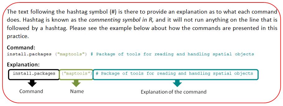
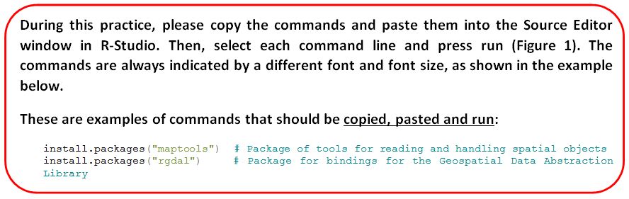
- In order to use these packages, they need to be loaded into the library, hence the presence of the library command after running install.packages. This command also needs to be run when restarting R-Studio. In addition, as the command to install.packages() is a character string, remember to insert the quotes around the package name. An example of this can be seen in Figure 1.
- To run the commands, please copy the commands presented in this practice into the Source Editor window. Select each command and click run, as illustrated in Figure 1.
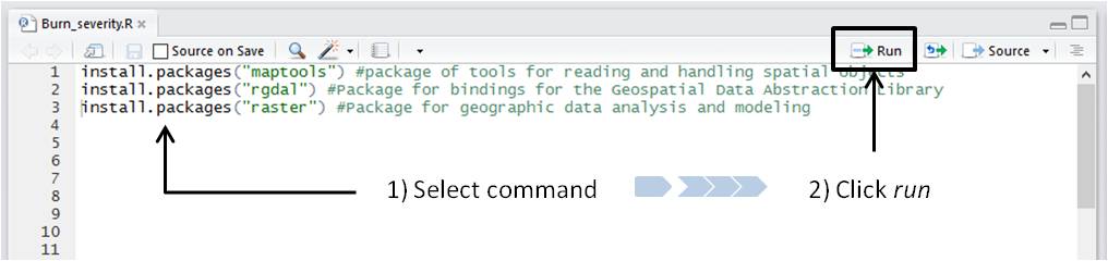
Figure 1. How to run a command in R-Studio.
- When a command is run, you should see the process update in the Console Window, which will also show if it has been successful or not.
- The path indicating the work directory needs to be updated to reflect the user’s working directory. Please note that if the path is copied and pasted using a Windows platform, the backslash ('\') must be replaced by a forward slash ('/'), as exemplified in Figure 2.
Figure 2. Illustration of the replacement of slashes for R-Studio to run.
- R-Studio does not automatically save your work environment, plots, or scripts. The user should therefore manually save them if desired.
- If after running the install.packages and library command there is an error such as the one shown in Figure 3, please re-install the corresponding package and run library again.
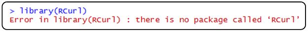
Figure 3. Example of an error whilst running the library command.
Part 2: Burn Severity
To start, please confirm that all data is in the same folder. To start processing, you should have the following files in the same folder. The files are listed below and the folder structure is shown in Figure 4.
- The pre-fire images (all bands in the same folder)
- The post-fire images (all bands in the same folder)
- The shapefile of the assessed area.
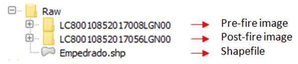
Figure 4. The file structure to enable processing.
1. Install Packages
A package is a directory of files used to perform a number of tasks in R; examples of which include a source package (the master files of a package), a .tar file containing the files of a source package, or an installed package (Rainey, 2013). Packages are basically collections of R functions, data, and compiled codes in a well-defined format, that are used in R to perform tasks.
2. Attach Packages into the Library
The directory where packages are stored is called the ‘library’. The ‘library’ is a directory into which the previous packages are installed. Please note: The same name is used to install the packages and to load them into the ‘library’.
At this point, your Source Editor window should look similar to the one shown in Figure 5.
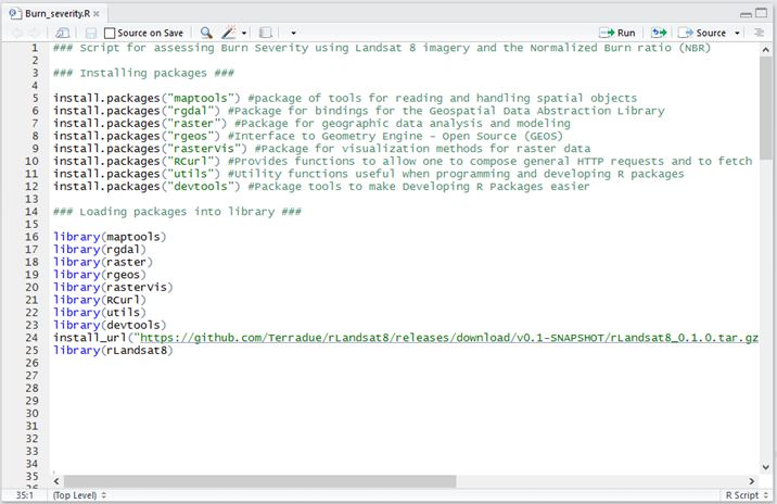
Figure 5. Screenshot of the Source Editor window.
3. Set the working directory
To begin, the working directory (where all your data is), needs to be assigned. For this, please run the following command:
THE PATH TO THE WORKING DIRECTORY (IN QUOTES) NEEDS TO BE REPLACED WITH THE USER’S WORKING DIRECTORY. PLEASE REMEMBER TO REPLACE THE SLASHES, AS SHOWN IN FIGURE 2.
4. Load the pre- and post-fire images
Bands 5 (NIR) and band 7 (SWIR2) of pre- and post-fire need to be loaded into the R environment. The date chosen to represent the pre-fire image during this practice was from 8th January 2017 and the post-fire was from 25th February 2017. To read a raster file in R-Studio, the function ReadLandsat8 is used and a new name is assigned to the product. For example, the names assigned for the pre- and post-fire images were lspre and lspost, respectively.
ReadLandsat8 is a function from the rLandsat8 package. This function reads the Landsat 8 products that are in the folder (i.e. it reads the metadata, and the bands in the correct order, without physically renaming them).
At this point, the windows in your R-Studio should look similar to those shown in Figure 6.
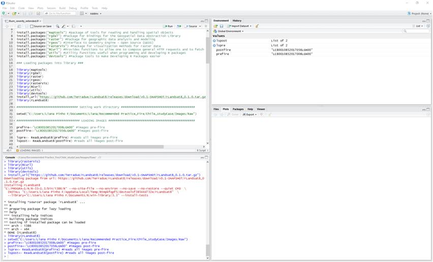
Figure 6. Screenshot of the processing done until now.
5. Correct images for Top of Atmosphere (TOA) reflectance
In order to calculate NBR, it is recommended that the images for the TOA reflectance be corrected. For more information on what TOA reflectance is, and why it is corrected, please refer to TOA reflectance.
To calculate the TOA corrections, the command ToTOAReflectance is run. It is normal for this part to take approximately 5 minutes to run, depending on the configuration of your computer. The commands are executed in the following way:
Your R-Studio windows should now look similar to those shown in Figure 7.
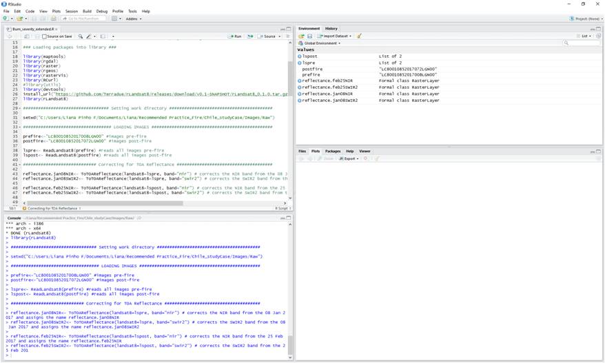
Figure 7. Screenshot of the processing done after running the reflectance corrections.
Tip: It is good practice to plot the images, in order to check they were loaded correctly. For this, the command plot is used, so the images are plotted in the bottom right window. The command to plot the NIR band from 8th January 2017 is shown below. Please note that the plotting process may take a few minutes.
After plotting, your R-Studio should look similar to that shown in Figure 8.
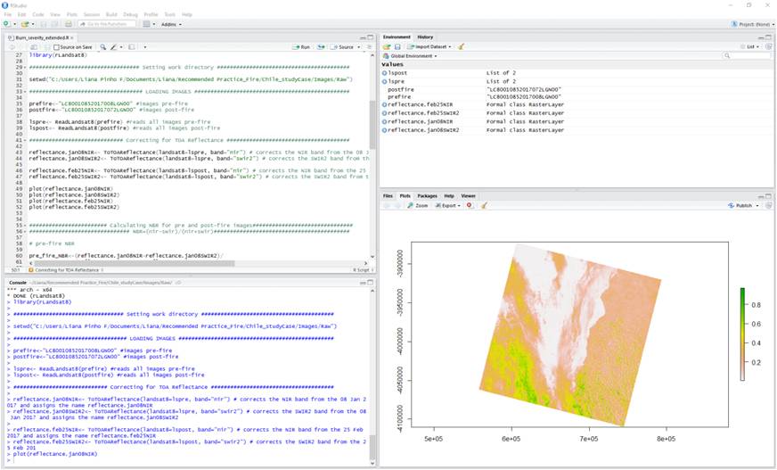
Figure 8. Screenshot of the processing done, including the plotted reflectance for 08 January 2017.
Please proceed to also plot the other images that were previously loaded. The commands to plot them are below. Please take into consideration that plotting may take a few minutes.
Keep in mind that they will be plotted in the bottom right window, but the images can be seen using the arrows indicated by the red box in Figure 9. The colors are, as per default, in R-Studio.
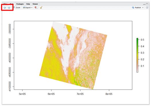
Figure 9. A plot of the image after the TOA correction. The red box indicates the arrows that can be used to scroll through the plotted images.
This step corrects the bands that are used to calculate NBR. Once they have been corrected, it is possible to calculate NBR.
To crop a raster in R-Studio, it is necessary to run two commands in sequence. The first command is to mask followed by the command to crop. The difference between masking and cropping can be seen in Figure 15. The commands may take a few minutes to run.
6. Calculate NBR for the pre- and post-fire images
NBR is calculated using the corrected NIR and the second SWIR of Landsat 8. The formula is:
NBR = (NIR-SWIR2) / (NIR+SWIR2)
For more information on the theoretical background of NBR, please click here. The commands to obtain NBR for both pre- and post-fire images are below. Each of the commands should take about 2 minutes to run.
Your workspaces should now look similar to those shown in Figure 10.
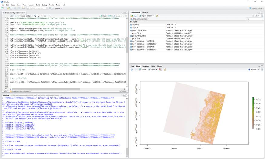
Figure 10. Screenshot of R-Studio illustrating the processing done up until now.
This then generates the Normalized Burn Ratio for the pre- and post-fire images. In order to assess the burn severity, it is necessary to calculate the difference between these two ratios (pre- and post-). For that, dNBR is calculated, as demonstrated during the next step.
7. Calculate dNBR (delta NBR)
The difference between the pre- and post-fire NBR maps is then calculated in order to obtain dNBR. dNBR is calculated using the following formula:
dNBR = (pre-fire NBR) - (post-fire NBR)
For more information about dNBR, please click here. The commands to obtain dNBR are as follow (this should take approximately 3 minutes to run):
Please note that the following warning message will appear on screen: ‘In (pre_fire_NBR) - (post_fire_NBR): Raster objects have different extents. Result for their intersection is returned’. As the result for the interested area has been returned, it is ok to continue.
The dNBR that will be used for burn severity has already been calculated. However, it has been calculated for the entire image. It is still necessary to crop the image to only reflect the study area: Empedrado, Chile.
8. Cropping the image
In order to crop the image, the shapefile "Empedrado.shp" must be loaded into R and named as Empedrado. As the coordinate system of the shapefile used and the corresponding images are different, the coordinate system of the shapefile needs to be altered to match the images’ coordinate system:
To crop a raster in R-Studio, it is necessary to run two commands in sequence. The first command is to mask followed by the command to crop. The difference between masking and cropping can be seen in Figure 11. The commands may take a few minutes to run:
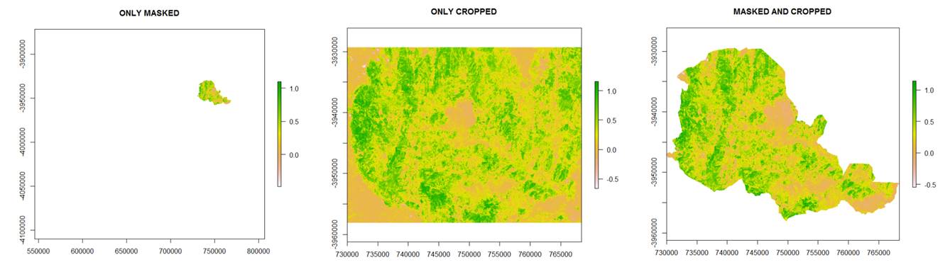
Figure 11. Comparison of the results obtained using the commands: mask, crop and mask followed by crop.
9. Classify the Burn Severity map
colour obtain the burn severity map, it is necessary to classify dNBR. The classification should be conducted in accordance with the USGS burn severity standards. The classifying process is carried out in a number of steps, as shown below:
10. Building the legend
Now that the burn severity map has been generated, the legend for the burn severity classes also needs to be created. The steps to create the legend are as shown:
Both the severity map and legend are now ready to use. However, the colours of the map are still set in default mode and should be changed to represent the burn severity properly.
11. Changing the plotted colours
In order to assess the burn severity, it is recommended to change the colours that were plotted in R-Studio, so it is visually clear. Now that the map and legend have been generated, you will change the colours of the map. There is no standardized colour palette, so you can choose the colours as you wish. The colours are assigned to the same sequence shown for the legend in step 10, i.e. 'white' is assigned for 'NA'; 'darkolivegreen' is assigned for 'Enhanced Regrowth, High', and so on.
The commands to change the colours and plot the map are:
The post-fire image used for this practice was obtained shortly after the fire had been extinguished. Therefore, there was no strong indication of regrowth in the study area, even though the legend shows otherwise (Figure 12). In order to analyze regrowth in the area, please follow the additional steps section.
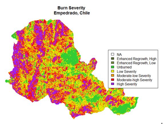
Figure 12. Burn Severity map of Empedrado, Chile.
12. Estimate the hectares of land destroyed by fire in each severity class
Estimating the total area of land destroyed is very important, also estimating the burnt area with respect to the classes burn severity is vital for the determination of the habitat loss based on the degree of damage done by a fire event.
| Country | Municipality | No data | Enhanced Regrowth-High | Enhanced Regrowth-Low | Unburned | Low Severity | Moderate-low Severity | Moderate-high Severity | High severity | |
| Fire period | Chile | Empedrado | 11.97 | 368.64 | 420.84 | 21624.57 | 2693.25 | 4119.48 | 5803.29 | 4447.08 |
| Reference period | Chile | Empedrado | 3.2 | 200..07 | 2100.78 | 27955.62 | 7164.36 | 1050.75 | 934.02 | 80.28 |
EXTRA STEPS
This section is dedicated to assessing the severity of burned areas whilst the fire was still active (for example, as in Chile the wildfire lasted for weeks, the same procedure could be used to assess the areas already burned).
SCENARIO: During the fire
1. Download image from 24th January 2017
To assess during fire, please download the images obtained on the 24th January 2017, matching the details shown below:
- Entity ID: LC80010852017024LGN00
- Coordinates: -36.04326, -73.04788
- Acquisition Date: 24-JAN-17
- Path: 1
- Row: 85
Figure 13 illustrates the satellite image from 24th January 2017 (true colour) that you should see.
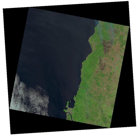
Figure 13. Landsat 8 true colour image from 24 January 2017.
2. Save the image in the same folder
To continue using the same script, it is necessary to save the images into the same folder you have been using throughout, i.e. where the working directory was set-upon step 3.
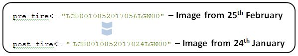
3. Load the new image to be assessed
Go back to STEP 4 of the recommended practice and replace the post-fire image assigned earlier as "LC80010852017056LGN00" with the image during the fire, as shown in the example below:
After running all the commands starting from step 4, you should now be able to see a similar map to the one shown in Figure 14.
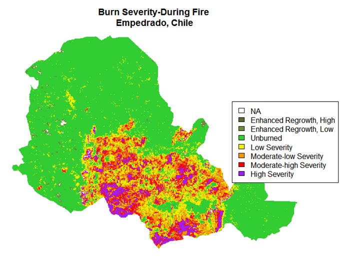
Figure 14. Burn Severity map before the fire was extinguished.
Please note that the burn severity assessment for when the fire was active should only be used as a reference; due to the fact that the intensity of the fire, and presence of smoke, could potentially interfere with the burn severity analysis.
You can also do the same process to assess the vegetation regrowth in the study area. For that, you can download the images weeks after the fire has been extinguished.