Step 1: Angular Normalization
Satellite-observed NTL radiance has a strong nonlinear relationship with the Viewing Zenith Angle (VZA), causing significant time-series fluctuations. This step normalizes the radiance as if the VZA is always zero.
1. Principle:
The angular normalization algorithm is designed to remove the variations in observed night-time light radiance derived from changes in the Viewing Zenith Angle (VZA). Previous research identified a strong nonlinear relationship between night-time light radiance and VZA, which can be expressed as:
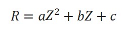
Where Z denotes the VZA, R denotes the night-time light radiance, and a, b, and c represent the coefficients. This model is called the Zenith-Radiance Quadratic (ZRQ) model.
The purpose of the normalization algorithm is to estimate the radiance time series assuming the VZA is equal to zero over time. Based on previous studies, we assume that the anisotropy of night-time light radiance remains constant if the land use of an area does not change over a short period. Therefore, the radiance in all directions will change by the same percentage even if the total light emission of the region changes. Based on this basic hypothesis, the radiance of night-time light over a period is modeled as:
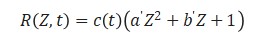
Where R (Z,t) epresents the night-time light radiance under the VZA of Z at moment t , c (t) is the actual radiance at moment t assuming the VZA is zero, (α'Z2 + b Z + 1) is the function changing with VZA, and α' and b' are the coefficients. This model effectively decomposes the satellite-observed time series radiance dynamic into two components: the real light emission changes (represented by the radiance at a VZA of zero, c(t) ), and the VZA-change-derived radiance observation due to the anisotropy.
2. Implementation Steps:
1) Define the Objective Function: The algorithm assumes that if land use remains unchanged, the anisotropy of NTL radiance remains consistent over a short period. The goal is to estimate the time series radiance c(t) at a VZA of zero. The objective function minimizes the correlation (R2) between the angle-normalized time series and the VZA using a Zenith-Radiance Quadratic (ZRQ) model.
2) Optimize and Solve:
- Utilize the Nelder-Mead algorithm to minimize the objective function and solve for the required coefficients.
- In Python, this can be implemented using the scipy.optimize.fmin package.
Image Source: Jia et al. 2023 https://doi.org/10.1016/j.jag.2023.103359
Step 2: Time Series Gap-Filling
After obtaining the angle-normalized time series T, we need to use an additive time series model named Prophet to gap-filling the missing data which makes the time series more complete.
The Prophet model is a generalized time series model that can handle various types of patterns, including seasonal and non-seasonal characteristics, which mainly includes the trend term, seasonal term, and the error term. The three terms are optimized by the L-BFGS algorithm to obtain the fitted value. We use the real observation data to fit the time series, and only fill in the fitted values of night-time light radiance at the missing moments thereby completing the time series gap-filling.
Due to the strict filtering criteria in the pre-processing stage (e.g., removing cloud or moonlight contaminated pixels), the resulting time series will have missing data points.
- Apply the Prophet additive time series model to fill in the missing gaps.
- The Prophet model handles seasonal and non-seasonal characteristics by optimizing trend, seasonal, and error terms using the L-BFGS algorithm. Fill in the fitted values only at the missing moments to complete the time series.
Step 3: Estimation of Power Restoration
Once the stable and continuous time series is generated, it can be used to assess disaster damage and track power recovery.
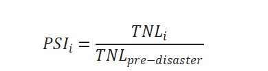
1. Power Supply Index (PSI): Calculate the PSI to quantify the current power supply relative to the pre-disaster baseline.
2. Power Restoration Index (PRI): Calculate the PRI to measure resilience and the chronological progression of recovery from the maximum point of damage.
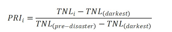
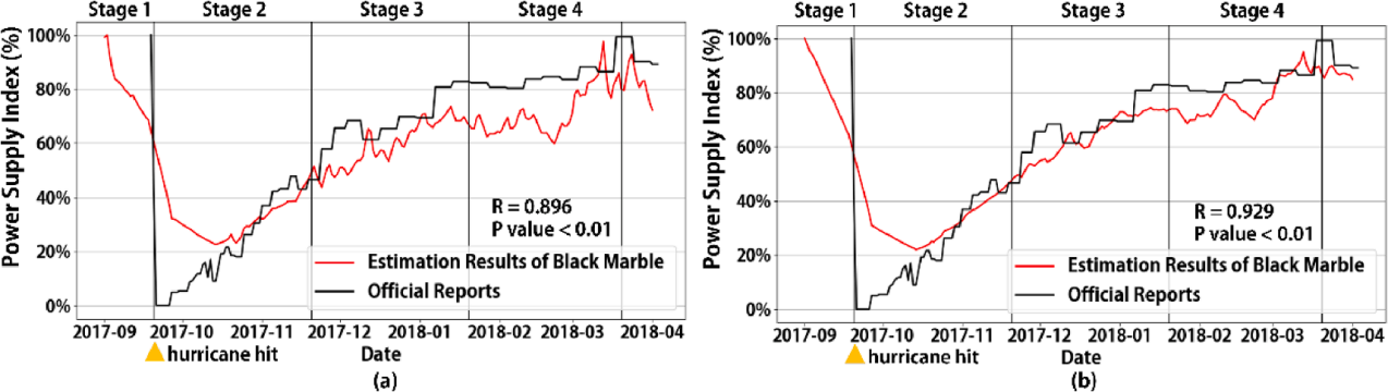
Image Source: Jia et al. 2023 https://doi.org/10.1016/j.jag.2023.103359