The aim of this step-by-step procedure is to create a standardized precipitation index (SPI) timeline based on daily CHIRPS data. The SPI is used as it highlights the difference to the mean precipitation during a given time and therefore provides information about drought-like conditions. The script will be executed within the Google Earth Engine and will work on two undependend SPI calculations. The first calculation deals with the "common" SPI, which is calculated on a n-months basis. A SPI, which is calculatet for one month usually referes to the description of "SPI-1", for six months "SPI-6" and so on. The second SPI calculation is based on MODIS's capture dates. As MODIS provides information about the vegetation, it might be useful to compare its vegetation idices with the SPI. Therefore a 16-day SPI is calculated, whose start date matches with MODIS's start date.
Google Earth Engine (GEE) is a web-platform for cloud-based processing of remote sensing data on a large scale. The advantage lies in its remarkable computation speed as processing is outsourced to Google servers. The platform provides a variety of constantly updated datasets; no download of raw imagery is required. While it is free of charge, one still needs to activate access to Google Earth Engine with a valid Google account. A confirmation is usually received within 2 to 3 working days. For a quick orientation around the code editor, please click here.
The code for this Recommended Practice can be imported by following this link.
1. Selecting an area of interest (AOI)
In the following section we will present three different ways to specify the location of your study area. This information is necessary to limit the processing extent of the analysis and avoids redundant calculations. Users can upload location information from a file, import country boundaries provided as GEE FeatureCollections or draw an area of interest by hand.
1.1 Shapefiles
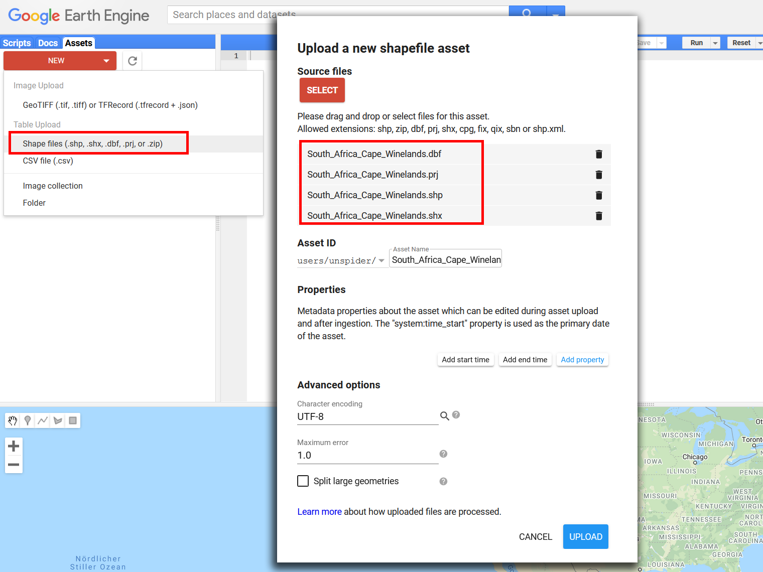
Defining the spatial processing extent with an ESRI-Shapefile (.shp) is the most accurate solution. This is recommended when researching a very distinct study area (e.g. a watershed). Start the import via the "Assets"-tab in the top left corner. On the "New"-drop-down menu select "Shape files'", then select your file. Careful: Make sure also to include the .dbf, .prj and .shx files, as the shapefile relies on them.
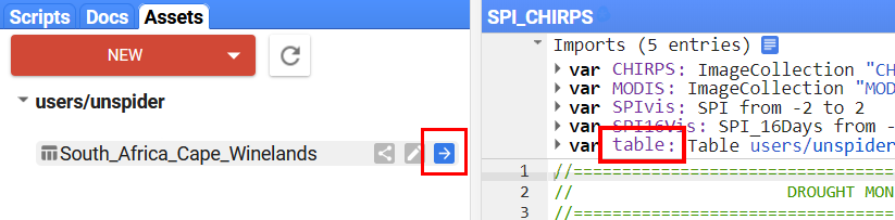
Uploading files usually takes a few minutes. You can observe the progress in the "Tasks"-tab on the top right. Once the "Asset ingestion"-task is completed (turns blue) you can import the shape to the script. You might have to refresh the assets tab in case your shapefile does not appear. Under "Assets" click the "Import"-button so the table is listed in the imports section. For the script to recognize this new shapefile, rename it to "AOI" (stands for "Area of Interest").
1.2 Built-in features
GEE so far provides a very limited amount of shapes such as administrative boundaries. If one seeks to perform this analysis on the country level though, there is a suitable data set provided that contains simplified features. In GEE, search for "LSIB'" or "International Boundaries". The FeatureCollection can be imported using its ID ("USDOS/LSIB_SIMPLE/2017"). Select a specific country by filtering the collection by FIPS country code. Here is an example for Costa Rica ("CS"):
var AOI= ee.FeatureCollection('USDOS/LSIB_SIMPLE/2017').filterMetadata('country_co', 'equals', 'CS');
Paste this line of code at the top of your script and make sure this is the only geometry variable in the script. Replace 'CS' with a country code of your choice.
1.3 Hand-drawn polygons
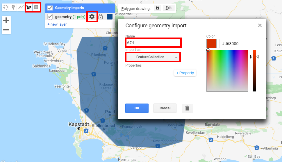
Besides uploading or importing location data, study area boundaries can be created interactively. This is the quickest and easiest option, suitable for exploring and testing the script in different regions. The polygon tool can be activated in the top-right corner of the map pane. Vertices are created with left clicks and the polygon is completed by double-clicking. A geometry can consist of more than one polygon. Once finished drawing the polygon open its setting by hovering over "geometry" in the "Geometry Imports". Change its name to "AOI" and its type to "FeatureCollection". The new AOI will be imported into the "Imports" section at the very top of the script.
2. Selecting a time frame
Besides the area of interest, the user is able to change the time scale of the calculations. This might not be necessary as the script gets the start and end date of the whole data collection and adapts its calculation according to the existing date range.
However, the resulting SVI values might get distorted if the start and end dates are changed, as a shortened lapse of time results in a reduction of the sample size for the calculations.
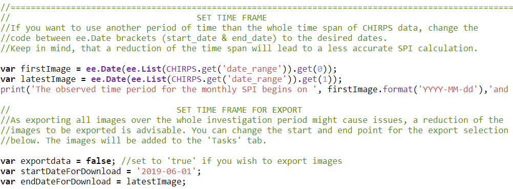
Beneath the start- and end date variables for the calculation timescale, you can find two variables concerning the start- and end date of the exported images. The export function itself has to be activated by setting it to "true". The strengths of the Google Earth Engine lie in the computing power, less so in the export of large image collections. Therefore, a reduction of the images to be exported or disabling the export function might be useful. Providing a timescale out of which you would like to download the SPI images will add those images to the "Tasks" tab.
3. Set processing resolution
CHIRPS data comes at a resolution of 0.05° which corresponds to approximately 5550 meter at the equator according to USNA. This figure is also set as the default resolution for the calculations, but it can be changed to any desired resolution. It might be usefull decresing the resolution when working on large AOI, as the GEE might face calculation timeouts otherwise. The resolution affects the calculations for the graphs in the console depicting the precipitation and SPI timelines and the resolution of the exported images. It does not affect the reolution of the images that are shown in GEE's map section.
4. Setting time steps
4.1 Time step for SPI on a basis of one to several months
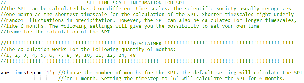
The first calculation deals with the "common" SPI and will be calculated for one or for several months. The observed number of months can be adjusted by changing the value behind the variable "timestep". For example: Setting the value to '6' will calculate the SPI on a six months basis counting backwards from the most recent date. It is not possible to calculate the SPI-12 (12 months SPI) with this script.
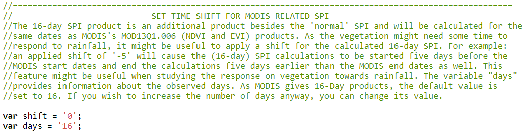
4.2 Time step MODIS related SPI
The second calculation deals with an SPI, whose dates are realted to MODIS's capture dates (the SPI is still based on CHIPRS data). This might help to compare precipitation with vegetation data. The user can apply a relative time "shift". This means that the start date of the SPI calculation is shifted relatively to MODIS's capture dates. A shift of '-5' will lead to an SPI image that starts five days earlier, but also ends five days earlier than the corresponding MODIS image. This might be useful when observing the reaction of the vegation to the precipitation. The default value is '0', which means that the start and end dates of the SPI matches with the start and end dates of MODIS's data. The next variable ("days") deals with the observed number of days for the SPI. The default value is set to '16' as this is the capture rythm of MODIS.
5. Obtaining additional information
It is possible to generate an additional chart in the lower right corner, which displays the timeline of the SPI-n of a specific location. The function is activated if the variable "showInteractiveChart" is set to 'true'. The chart will appear if a location within the AOI is being clicked.
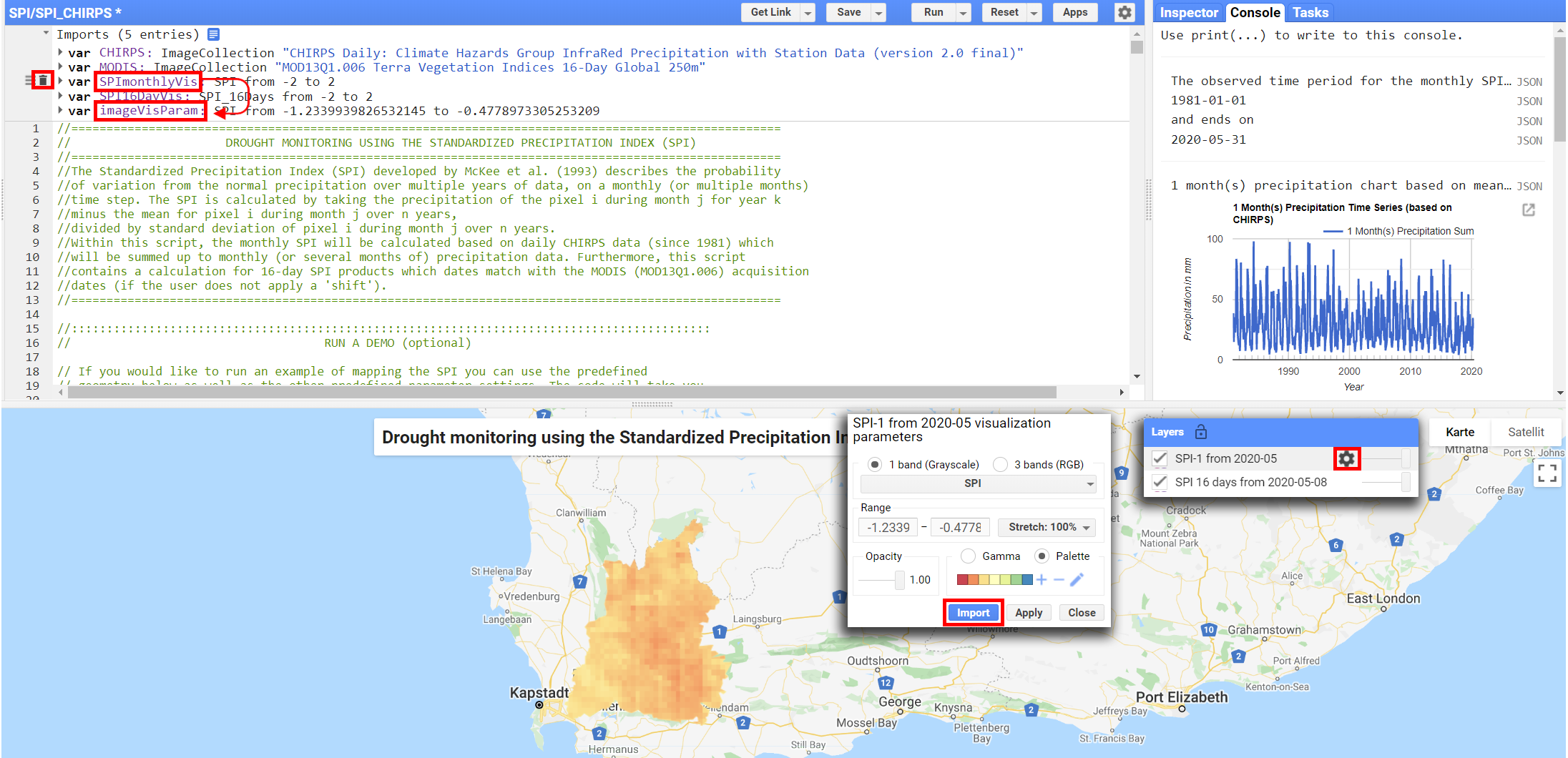
After finishing the calculations, Google Earth Engine will display the latest SPI-n image, as well as the latest MODIS related SPI image in the map section. You can toggle the visualization of the two layers by hovering over "Layers" and (de-)activating their checkboxes. A visual comparison of the layers can be conducted by using the sliders. In order to receive a pixel value from the visualized images go to the "Inspector" tab and click on a location within you AOI. The additional inspector chart will then also appear (if not deactivated in the script).
The charts, which are printed into the "Console" display the precipitation, the SPI-n and the MODIS related SPI over time by taking the mean of all pixels in your AOI for each acquisition date. A positive SPI indicates an above-average precipitation for the specific period. A negative SVI indicates a below-average precipitation for the specific period.
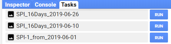
Downloading the results might be inevitable for further analysis. However, as mentioned above, downloading large image timelines is not one of Google Earth Engine's strengths. Should you want to download the images, you can start the download of the images by selecting the "Run" button of each filename within the "Tasks" tab. It is possible to start all tasks at the same time by using this script. The naming of the files follows this scheme:
Limitations
The legends pick their maximum and minimum values from the visualization parameters in the "Imports" section. If you wish to adapt the numbers in the legend to a new visualization layout, you have to import the new settings to the script, delete the old visualization parameters and rename the new parameters to the same name as the old ones before re-running the script.