The aim of this step-by-step procedure is the generation of a flood extent map for the assessment of affected areas. The flood extent is created using a change detection approach on Sentinel-1 (SAR) data. To assess the number of potentially exposed people, affected cropland and urban areas, additional datasets will be intersected with the derived flood extent layer and visualized.
The following step-by-step procedure uses Google Earth Engine, which is a powerful web-platform for cloud-based processing of remote sensing data on large scales. The advantage mainly lies in its computational speed, as processing is outsourced to Google’s servers. The platform provides a variety of constantly updated datasets which can be accessed directly within the code editor. No download of raw imagery is required. While it is free of charge, an activate Google account with Google Earth Engine is required. A confirmation usually comes within 2-3 work days. For a quick orientation around the code editor, click here: https://earthengine.google.com/platform/.
The code for this Recommended Practice can be imported by following this link:
https://code.earthengine.google.com/f5c2f984c053c8ea574bfcd4040d084e.
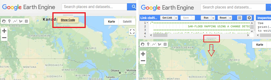
Fig. 1: Access the Google Earth Engine script by using the link.
There you will find detailed comments along with the code line-by-line. Alternatively, you can create a new file in the code editor, download this script and paste it.
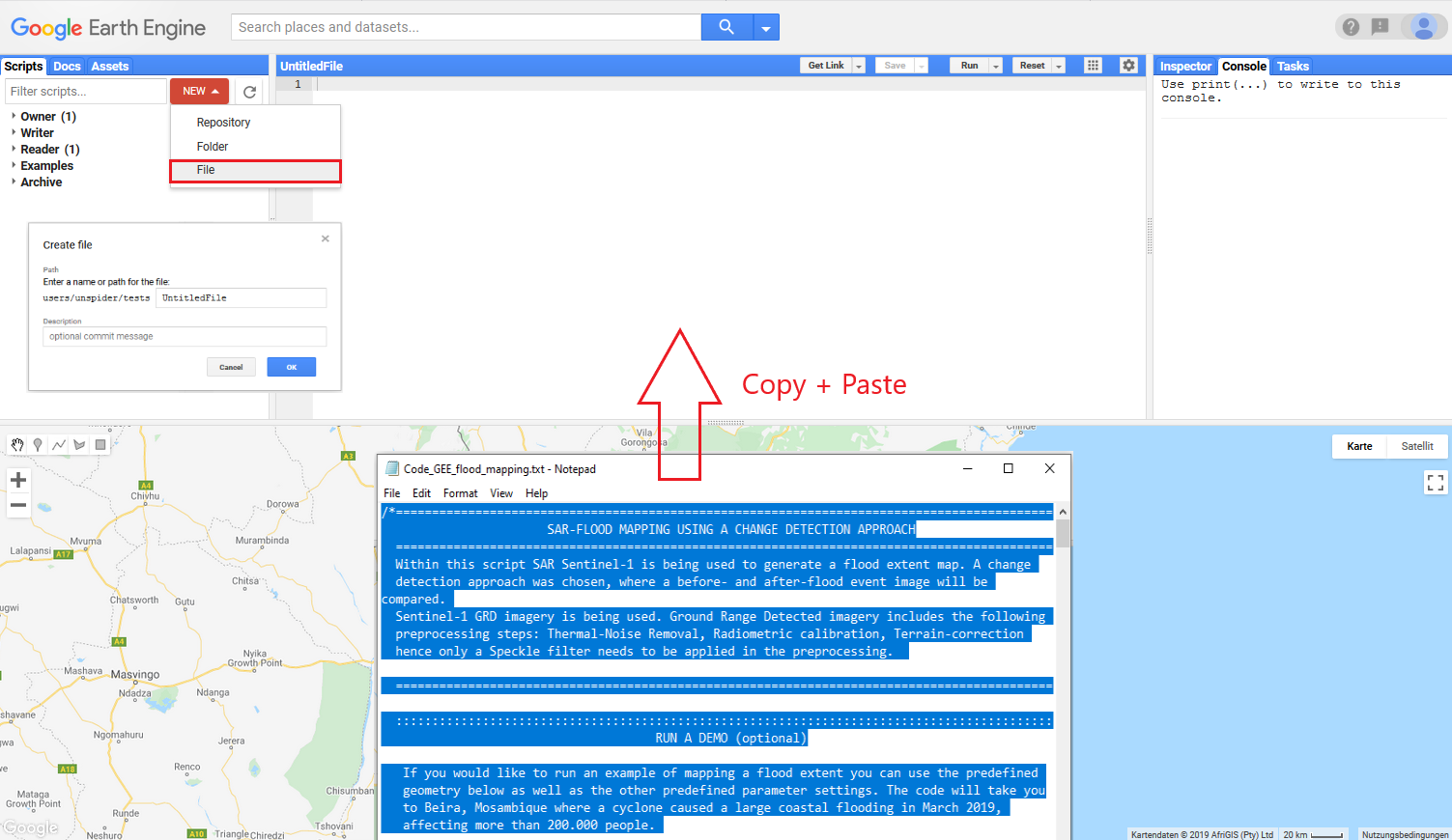
Fig.2: Access the Google Earth Engine script by copy-and-pasting the text-file.
Content:
Step 2: Time frame and sensor parameters selection
Step 4: Visualize results in GEE
Step 9: Refining the flood extent layer
Step 10: Area calculation of flood extent
Step 1: Study area selection
In the following section we will present three different ways to specify the location of your study area. This information is necessary to limit the processing extent of the analysis and avoids redundant calculations. Users can draw an area of interest by hand, upload location information from a file or import country boundaries provided as GEE FeatureCollection.
Boundaries can be created interactively. This is the quickest and easiest option, suitable for exploring and testing the script in different regions. The polygon tool can be activated in the top-right corner of the map pane. Vertices are created with left clicks and the polygon is completed by double-clicking. A geometry can consist of more than one polygon. Press 'Exit' once you are done setting up your study area. The geometry will be listed under 'Imports' at the top of the script.
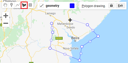
Fig. 3: Draw a polygon of the area of interest (aoi) by hand.
Defining the spatial processing extent with a Shapefile (.shp) is the most accurate solution. This is recommended when researching a very distinct study area (e.g. a watershed). Start the import via the 'Assets'-tab in the top left corner. On the 'New' drop-down menu select 'Table upload', then select your file. Careful: Make sure also to include the .dbf and .shx files, as the shapefile relies on them.
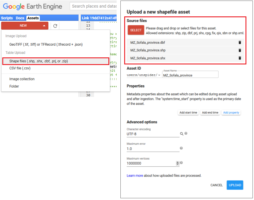
Fig. 4: Upload a shapefile to specify the area of interest.
Uploading files usually takes a few minutes. You can observe the progress in the 'Tasks’ tab on the top right. Once the 'Asset ingestion' task is completed (turns blue) you can import the shape to the script. Under 'Assets' click the 'Import' button so the table is listed in the imports section. For the script to recognize this new table, rename it to 'geometry'.
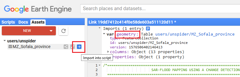
Fig. 5: Import the uploaded shapefile into the Google Earth Engine script.
1.3 In-build country boundary features
GEE so far provides a very limited amount of shapes, such as major administrative boundaries. If one seeks to perform this analysis on country level though, there is a suitable data set provided that contains simplified features. In GEE, search for 'LSIB' or 'International Boundaries'. The FeatureCollection can be imported using its ID ('USDOS/LSIB_SIMPLE/2017'). Select a specific country by filtering the collection by FIPS country code. Here is an example for Mozambique ('MZ'):
var geometry = ee.FeatureCollection('USDOS/LSIB_SIMPLE/2017').filterMetadata('country_co', 'equals', 'MZ');
Paste these lines of code at the top of your script and make sure this is the only geometry variable in the script. Replace 'MZ' with a country code of your choice.
Step 2: Time frame & sensor parameters selection
Besides the area of interest, the user is required to define pre- and post-flood time periods in the first few lines of the code. By setting periods, not single dates, the user allows the selection of enough tiles to cover the area of interest. Sentinel-1 imagery is acquired minimum every 12 days for each point on the globe (Figure 6).
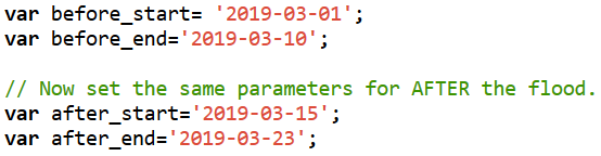
Fig. 6: Google Earth Engine Script for pre- and post-flood dates.
Furthermore, the user can choose between ‘VH’ and ‘VV’ polarization to perform the analysis. ‘VH’ is widely suggested for flood mapping, since it is more sensitive to changes on the land surface, while ‘VV’ is rather susceptible to vertical structures and might be useful to delineate open water from land surface (e.g. shoreline detection or a large water body that occurred after a flood event).

Fig. 7: Google Earth Engine Script for polarization
When performing change detection, it is necessary to select the same pass direction for the images being compared to avoid false positive signals caused by differences of the viewing angle. The user might choose between ‘DESCENDING’ and ‘ASCENDING’ pass direction, depending on the study area. As shown in Figure 9 some areas are only covered by descending pass directions (e.g. Brazil) or only by ascending (e.g. Namibia). Other areas, such as Mozambique or entire Europe are covered by both.

Fig. 8: Google Earth Engine Script for pass direction
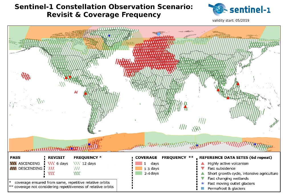
Fig. 9: Revisit and coverage frequency of the Sentinel-1 constellation, showing which areas are mainly covered with descending or ascending imagery. Source: https://sentinel.esa.int/web/sentinel/missions/sentinel-1/observation-scenario
To check whether the area of interest is covered given the selected parameters, expand ‘Layers’ in the top-right corner of the map viewer and select ‘After Flood’ as well as ‘Before Flood’.
Change the parameters ‘time frame’ and ‘pass_direction’ if your area of interest is not entirely covered!
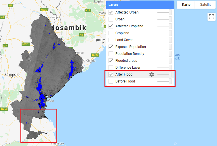
Fig.10: Expand ‘Layers’ and explore the coverage of your selected tiles for the before- and after flood mosaic. A part of the area of interest is not covered given the selected parameters.
Step 3: Run the script
When all parameters are selected hit ‘Run’ and wait for a few minutes until your results are displayed.
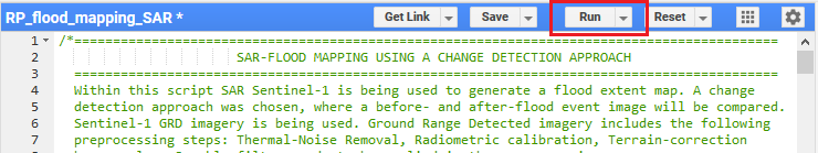
Fig. 11: ‘Run’- button to execute the script.
Step 4: Visualize results in GEE
Select the full-screen button in the top-right corner of the map viewer to visualize the flood product. Within ‘Layers’ you can check or uncheck the layers you are interested in and take a screenshot of the map as a first overview.
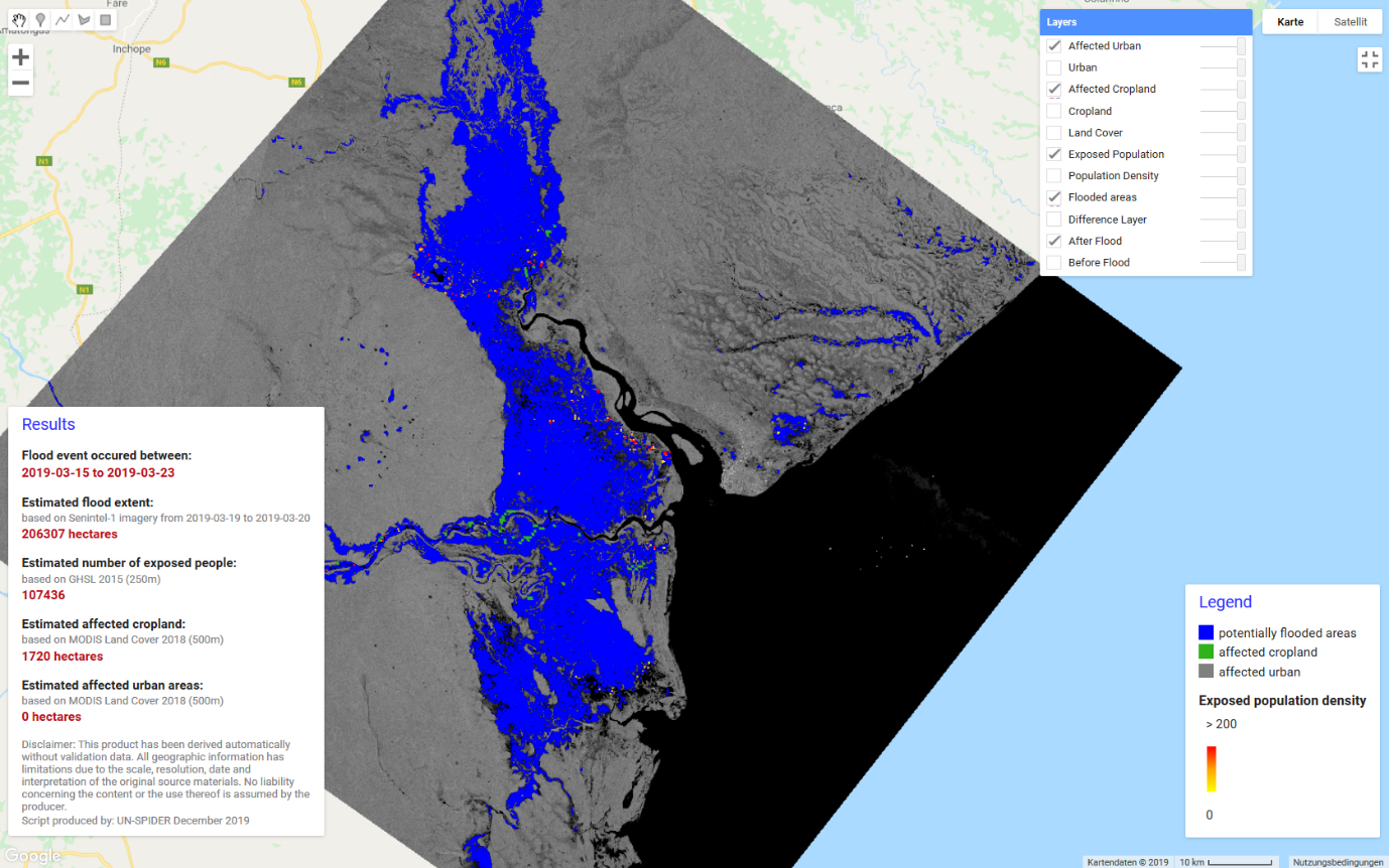
Fig. 12: Full-screen view of the results in Google Earth Engine map viewer.
Step 5: Export products
To export the generated products into your Google Drive account, click on ‘Tasks’ in the top-right corner of the code editor and hit ‘RUN’, and choose where to save the file. ‘Flood_extent_raster’ outputs a GeoTiff raster file of the flood extent. ‘Flood_extent_vector’ is a shapefile, where the flood extent has already been converted to polygons, which might be useful for further analysis. ‘Exposed_population’ includes a raster layer, showing the location and number of potentially exposed people.
This section explains the processing steps, which are performed automatically when running the Google Earth Engine script. It is recommended to read through them in order to understand how the data is being processed, which auxiliary datasets are used and what limitations the analysis may have for individual cases.
Step 6: Data filtering
According to the predefined parameters the entire Sentinel-1 GRD archive, called ImageCollection in Google Earth Engine, is filtered by the instrument mode, the polarization, pass direction, spatial resolution and are clipped to the boundaries of the area of interest. The filtered ImageCollection is then reduced to the selected time periods (before and after the flood event).
Step 7: Preprocessing
Information from Sentinel-1 Level-1 Ground Range Detected (GRD) imagery in Google Earth Engine has already undergone the following preprocessing steps:
- Apply-orbit-file (updates orbit metadata)
- ARD border noise removal (removes low intensity noise and invalid data on the scene edges)
- Thermal noise removal (removes additive noise in sub-swaths)
- Radiometric calibration (computes backscatter intensity using sensor calibration parameters)
- Terrain-correction (orthorectification)
- Conversion of the backscatter coefficient (σ°) into decibels (dB)
Hence, the code in this Recommended Practice only applies a smoothing filter to reduce the inherent speckle-effect of radar imagery (Fig. 13).
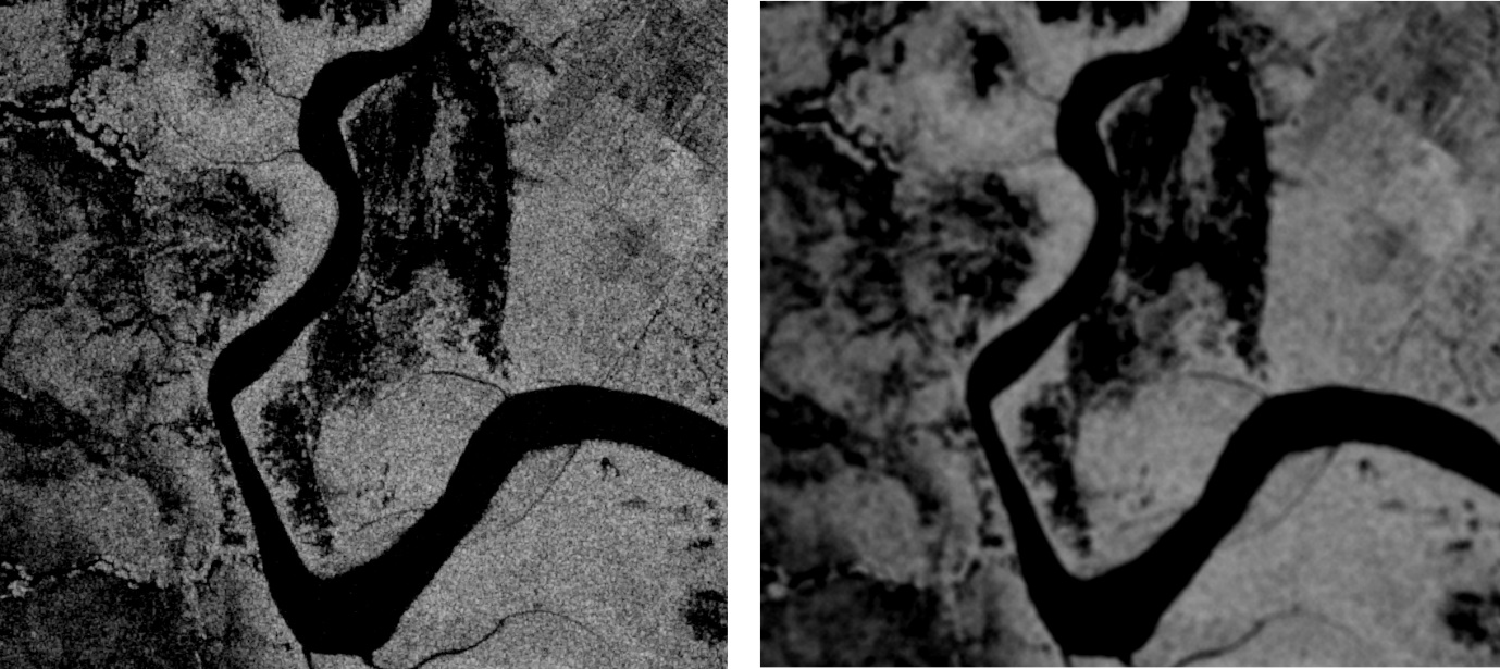
Fig. 13: Left: without smoothing. Right: applied smoothing of 50 m circles.
Step 8: Change detection
This script uses a simple, straight-forward change detection approach, where the after-flood mosaic is divided by the before-flood mosaic, resulting in a raster layer showing the degree of change per pixel. High values (bright pixels) indicate high change, low values (dark pixels) point toward little change. The predefined threshold of 1.25 is applied assigning 1 to all values greater than 1.25 and 0 to all values less than 1.25. The binary raster layer created by this process shows the potential flood extent (Fig. 14). The threshold of 1.25 has been selected through trial and error and might be adjusted in case of high rates of false positive or false negative values.
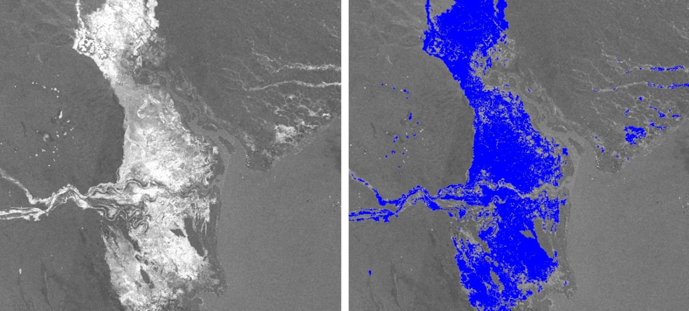
Fig.14: Left: difference layer, bright areas indicate high change, dark areas little change. Right: resulting flood extent layer by applying a threshold of 1.25.
Step 9: Refining the flood extent layer
Several additional datasets are used to eliminate false positives within the flood extent layer. The JRC Global Surface Water dataset is used to mask out all areas covered by water for more than 10 months per year. The dataset has a resolution of 30 m and was last updated in 2018.
To remove areas with over 5 % slope, a digital elevation model (WWF HydroSHEDS) has been chosen, which is based on SRTM data, and has a spatial resolution of 3 arc-seconds. Furthermore, the connectivity of the flood pixels is assessed to eliminate those connected to eight or fewer neighbors. This operation reduces the noise of the flood extent product (Fig. 15).
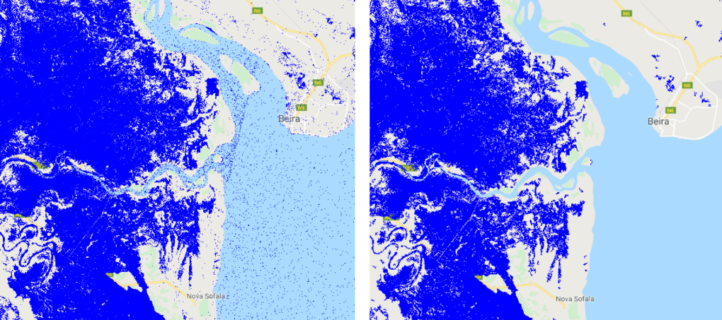
Fig.15: Left: original flood extent. Right: refined flood extent layer
Step 10: Area calculation of flood extent
To compute the area of the flood extent, a new raster layer is created calculating the area in m2 for each pixel, taking the projection into account. By summing up all pixels, the area information is derived and converted into hectares. The result is displayed on the ‘Results’ panel in the bottom-left corner of the Map Viewer.
Step 11: Exposed population density
To estimate the number of exposed people, the code uses the JRC Global Human Settlement Population Layer, which has a resolution of 250 m, and was last updated in 2015. It contains information on the number of people living in each cell. To intersect the flood layer with the population layer, the flood extent raster first needs to be reprojected to the resolution and projection of the population dataset. Subsequently, an intersection between both layers is computed and displayed as a new raster layer (Fig. 16 right). To calculate the number of exposed people, all pixel values of the exposed population raster are summed up and displayed in the ‘Results’ panel on the Map Viewer.
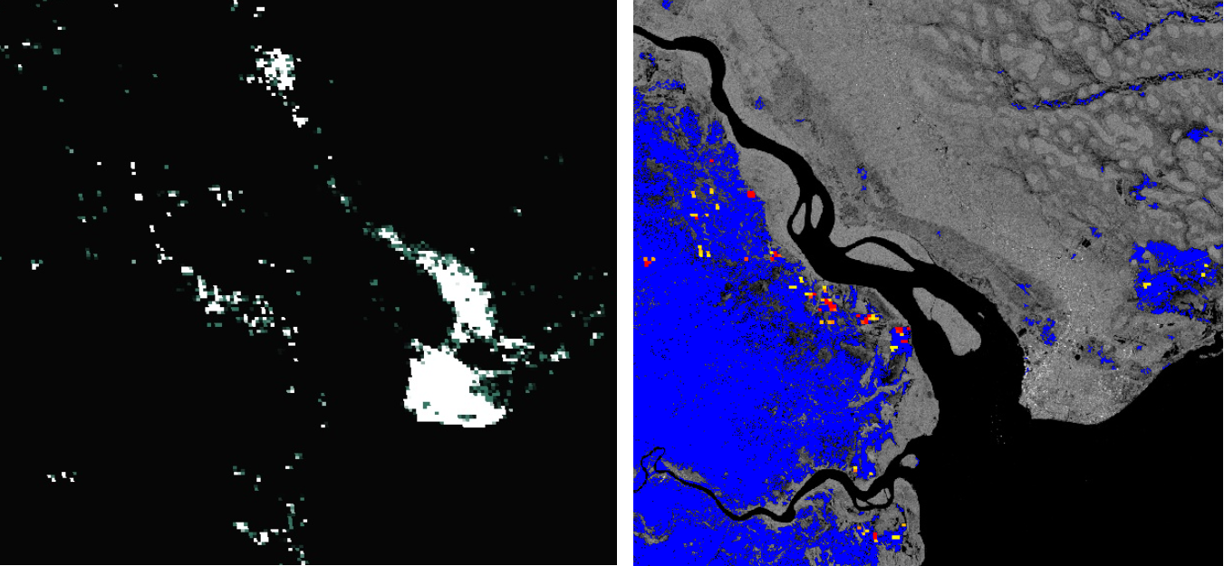
Fig.16: Left: Population density layer, the brighter the pixel the denser populated. Right: Population density exposed to the flood event (from yellow-red).
Step 12: Affected cropland
To estimate the amount of affected cropland, the MODIS Land Cover Type product has been chosen. The dataset has a spatial resolution of 500 m and is updated yearly. It is the only global dataset on Land Cover currently available in Google Earth Engine. The Land Cover Type 1 band consists of 17 classes with two cropland classes (class 12: at least 60% of area is cultivated and class 14: Cropland/ Natural Vegetation Mosaics: small-scale cultivation 40-60% with natural tree, shrub, or herbaceous vegetation). Both classes are extracted from the dataset and intersected with the flood extent layer, which has been resampled to the scale and projection of the MODIS layer (Fig. 17).
The area of the affected cropland is calculated the same way as for the flood extent and displayed in the ‘Results’ panel.
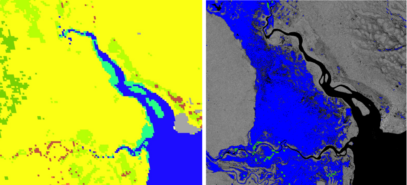
Fig. 17: Left: MODIS Land Cover (blue: water, yellow: savanna, dark green: forest, light green: grassland, turquoise: wetlands, grey: urban, red: croplands). Right: affected cropland in green
Step 13: Affected urban areas
Affected urban areas are calculated the same way as the previous two steps, using the MODIS Land Cover Type dataset. The ‘Urban Class 13’ of the band ‘Land Cover Type 1’ is extracted to assess potentially affected urban areas. In this process, affected urban areas are very likely to be underestimated, due to the difficulties of detecting water in build-up areas. See Strengths and Limitations for further details.