This page provides the step-by-step instructions to apply a multi-temporal analysis of the MODIS-based Standardized Vegetation Index (SVI) for large areas using R. Depending on the extent of the study area and the hardware capacities of the computer, the user might experiece difficulties applying this R script. We therefore provided an additional R script to be able the compute the VCI and monitor the vegetation conditions for large areas (>200.000km2) which can be accessed here.
For this Recommended Practice for drought monitoring we use the Enhanced Vegetation Index (EVI) based on MODIS data at 250m spatial resolution as input for generating theStandardized Vegetation Index (SVI). The only MODIS product providing EVI data is MOD13Q1 (on Terra satellite) and MYD13Q1 (on Aqua Satellite). MODIS data is for example made available on the Application for Extracting and Exploring Analysis Ready Samples (AppEEARS) by USGS.
If the Normalized Difference Vegetation Index (NDVI) is preferred for calculating the SVI, the EVI can easily be replaced with the NDVI as this product is also available for download at AppEEARS. Given this case, the caption of the resulting jpg maps should be adjusted. However, in certain circumstances, the SVI based on the NDVI does not perform as well as based on the EVI. See the "In Detail" page for more information.
For this recommended practice we use the Enhanced Vegetation Index (EVI) based on MODIS data at 250m spatial resolution as input. The only MODIS product providing EVI data is MOD13Q1 (on Terra satellite) and MYD13Q1 (on Aqua satellite).
Data and Software required for this Recommended Practice are:
- EVI and Pixel Reliability provided by MOD13Q1 (see next section)
- Shapefile of area of interest (https://gadm.org/country)
- R and R-Studio
![]()
If not yet installed, the R software and R-Studio can be downloaded here. To follow a step by step instruction on how to download and install R and R-Studio, please click here.
Content
Part A: Data preparation
- Step 1: Download MODIS data
- Step 2: Renaming and structuring of the data
Part B: Processing
- Step 3: Download R code
- Step 4: Adjust the script
- Step 5: Run the R Code
- View the Code
Part C: Results
Step 1 Download MODIS data as Geotiffs from AppEEARS
Access the AppEEARS website and create a user account (free) in case you do not already have one (https://lpdaacsvc.cr.usgs.gov/appeears/). Click on Extract and Area Sample and start a new request.
- Enter a request name
- Define your region of interest by specifying a ESRI shapefile (zip) or drawing a polygon . Country shapefiles can be downloaded at https://gadm.org/country. Note: The boundaries and names of the shapefiles do not imply official endorsement or acceptance by the United Nations.
- Define the time period of your data: January 2000 to today.
- Select the product: MOD13Q1 and the layers of interest: EVI and pixel_reliability
- Define the output as geotiff with geographic Projection
- Click on Submit


Click on Explore to check the status of the request. Click on the Download symbol once the status says Done. Select all ordered datasets and start downloading the data.

After the download store the files (.tif) in two folders: one folder for the Data_EVI and one for the Data_Pixel_Reliability. It is recommended to use an external hard drive to store your input and output data if possible.
Step 2 Renaming and Structuring of the data
For processing this Recommended Practice in R, it is required to first rename and second sort the data according to their DOY. Download the folder structure here and copy it both in the folders Data_EVI and Data_Pixel_Reliability.
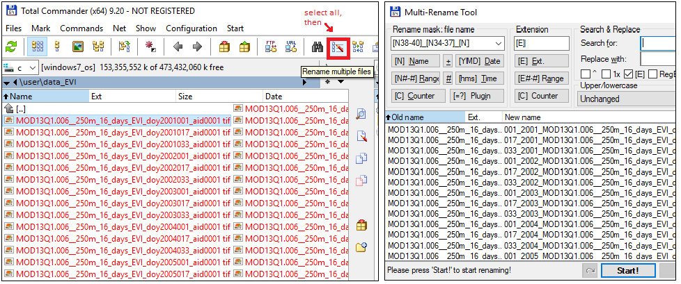
- Rename the EVI and pixel reliability data following the pattern: DOY_YYYY_[Original Name]. It is recommended to use Total Commander to rename multiple files (Download Link: http://www.ghisler.com/index.htm). Renaming the files is important because this pattern is used to automatize the filenames and the titles of the resulting maps in the R script.
- Sort the EVI and Pixel Reliability data according to the DOY in the respective folders.
Create following folders in addition to Data_EVI and Data_Pixel_Reliability:
- "shape" (store the shapefile with the country border here including .shp, .dbf, .prj, and .shx files)
- "SVI_Maps_jpg"
- "SVI_Maps_tif"

Step 3 Download R Code
Download the R Code here (right click and choose "save as"). The R Code is tailored to MOD13Q1 tif data.
Step 4 Adjust the script
Open R Studio and the saved R script (File -> Open File). The script needs various adjustments to fit your data. Note hereby: R uses slashes ("/") for file names and directories and not backslashes ("\").
- In line 23: border <- shapefile("C:/User/MOD13Q1/Data/shape/gadm36_GTM_0.shp") --- replace the data path by the data path and/or name of the shapefile that you have stored on your computer
- In line 26: path <- "C:/User/MOD13Q1/Data/Data_EVI" --- enter link to the folder where you have stored the MODIS EVI data
- In line 29: path_c <- C:/User/MOD13Q1/Data/Data_Pixel_Reliability" --- enter link to the folder where you have stored the MODIS Pixel Reliability data
- In line 32: path_jpg <- "C:/User/MOD13Q1/Data/SVI_Maps_Guatemala_jpg" --- enter the link to the folder where you want to store the resulting .jpg-images
- In line 33: path_tif <- "C:/User/MOD13Q1/Data/SVI_Maps_Guatemala_tif" --- enter the link to the folder where you want to store the resulting .tif-files
- In line 115: plot(SVI_all[[k]], # zlim=c(0,100), breaks=c(-4, breaksSVI[x], 4),col=colorsSVI, main=paste("SVI"," (EVI)"," Guatemala ",doy," ",year,sep="")) --- Adjust the country and file naming according to the data you are processing (e.g. if you base your SVI on NDVI, change to (NDVI))
Step 5 Run the R code
Install the raster, rgdal and sp packages by highlighting the respective text in the code and clicking on "Run" or typing Ctrl+Enter.

Now, run the remaining code by highlighting it and typing CRT+Enter. Depending on the size of your data, it will take quite a while (up to several hours) for the script to run - so be patient. After a while, a progress bar will be displayed in the console. Be patient, it might take a while for the progress bar to appear. It looks like this:
======
Note: Delete the temporary files of your computer and set the memory limit within R (memory.limit()) according to your free working memory for improving your computer's capacity to process the data.
View the Code
You can access the code on https://rpubs.com/
Part C Results
The results will be stored in the respective folders as jpg (SVI_Maps_jpg) and as tif file (SVI_Maps_tif) within your main directory. The maps are named "DOY_YYYY". The title of the jpeg maps is following the pattern "DOY SVI (EVI) YYYY", where DOY and YYYY are automatically adjusted according to the input data and (NDVI) can be adjusted manually in the script (see above). See below an example of the resulting jpeg map.

The SVI values represent how many standard deviations the present state of vegetation differs from the EVI mean in a specific pixel.
For this sample of 26 June 2018 (DOY 177), the EVI value in each pixel is compared to the EVI mean of DOY 177 from 2000 to 2018 in the respective pixel. The scalebar to the right shows the positive and negative deviations of pixels to the EVI mean with green highlighting positive deviations and red highlighting negative deviations. The vegetation in areas colored in yellow on the other hand have been identified with an average vegetation condition. White pixels have been masked out due to cloud/snow coverage or missing data within of the Pixel Reliability.
The SVI provides a useful analysis tool for the assessment of vegetation trends and monitoring of areas affected by drought. However, it cannot be used to quantify the magnitude of a drought hazard. Read more about the key strengthts and limitations of the SVI as well as its statistical background here.