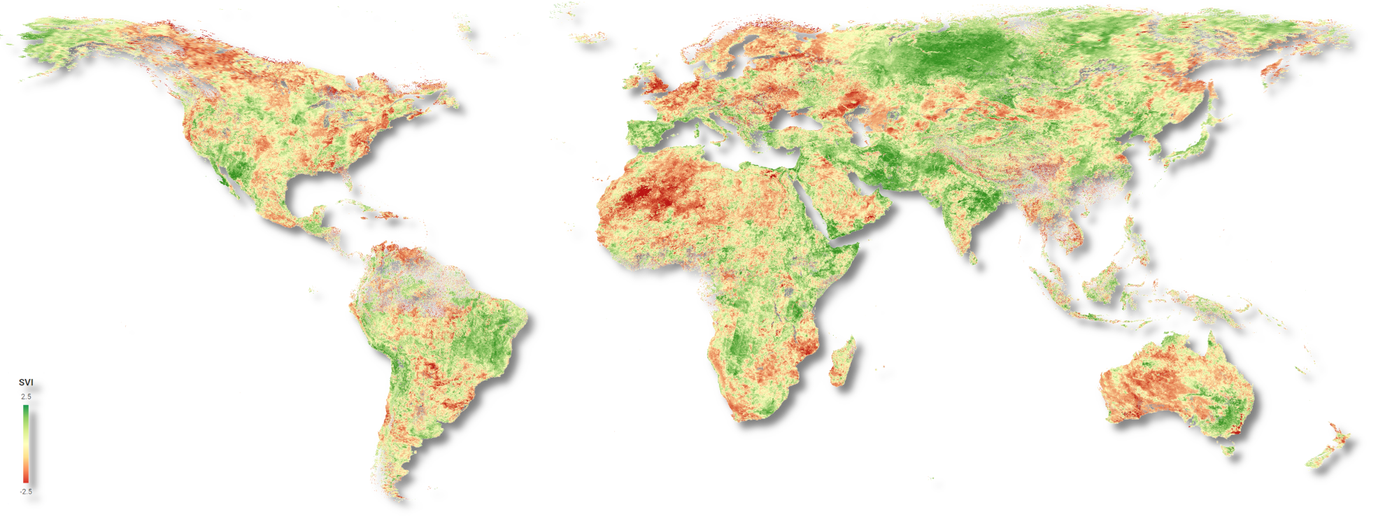
The aim of this step-by-step procedure is to create a standard vegetation index (SVI) timeline based on the MODIS enhanced vegetation index (EVI) product. The SVI is used as it highlights the difference to the mean vegetation status during a given time and therefore provides information about drought-like conditions.
Google Earth Engine (GEE) is a web-platform for cloud-based processing of remote sensing data on a large scale. The advantage lies in its remarkable computation speed as processing is outsourced to Google servers. The platform provides a variety of constantly updated datasets; no download of raw imagery is required. While it is free of charge, one still needs to activate access to Google Earth Engine with a valid Google account. A confirmation is usually received within 2 to 3 working days. For a quick orientation around the code editor, please click here.
The code for this Recommended Practice can be imported by following this link.
1. Selecting an area of interest (AOI)
In the following section we will present three different ways to specify the location of your study area. This information is necessary to limit the processing extent of the analysis and avoids redundant calculations. Users can upload location information from a file, import country boundaries provided as GEE FeatureCollections or draw an area of interest by hand. These three options as well as all other processing steps are explained in the video tutorial above.
1.1 Shapefiles
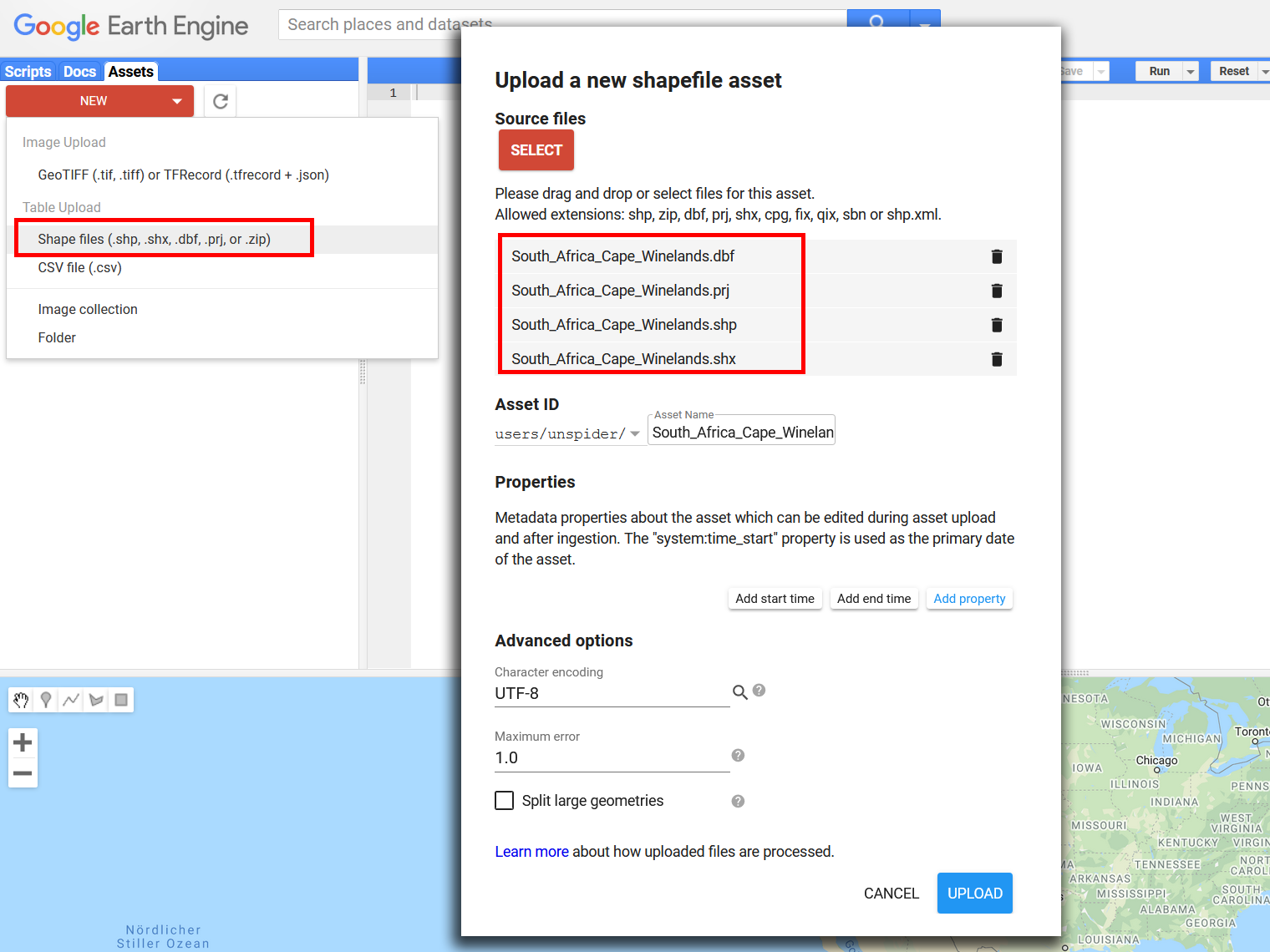
Defining the spatial processing extent with an ESRI-Shapefile (.shp) is the most accurate solution. This is recommended when researching a very distinct study area (e.g. a watershed). Start the import via the "Assets"-tab in the top left corner. On the "New"-drop-down menu select "Shape files'", then select your file. Careful: Make sure also to include the .dbf, .prj and .shx files, as the shapefile relies on them.
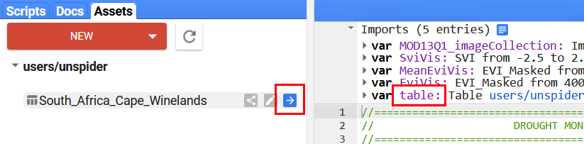
Uploading files usually takes a few minutes. You can observe the progress in the "Tasks"-tab on the top right. Once the "Asset ingestion"-task is completed (turns blue) you can import the shape to the script. You might have to refresh the assets tab in case your shapefile does not appear. Under "Assets" click the "Import"-button so the table is listed in the imports section. For the script to recognize this new shapefile, rename it to "AOI" (stands for "Area of Interest").
1.2 Built-in features
GEE so far provides a very limited amount of shapes such as administrative boundaries. If one seeks to perform this analysis on the country level though, there is a suitable data set provided that contains simplified features. In GEE, search for "LSIB'" or "International Boundaries". The FeatureCollection can be imported using its ID ("USDOS/LSIB_SIMPLE/2017"). Select a specific country by filtering the collection by FIPS country code. Here is an example for Costa Rica ("CS"):
var AOI= ee.FeatureCollection('USDOS/LSIB_SIMPLE/2017').filterMetadata('country_co', 'equals', 'CS');
Paste this line of code at the top of your script and make sure this is the only geometry variable in the script. Replace 'CS' with a country code of your choice.
1.3 Hand-drawn polygons
Besides uploading or importing location data, study area boundaries can be created interactively. This is the quickest and easiest option, suitable for exploring and testing the script in different regions. The polygon tool can be activated in the top-right corner of the map pane. Vertices are created with left clicks and the polygon is completed by double-clicking. A geometry can consist of more than one polygon. Once finished drawing the polygon open its setting by hovering over "geometry" in the "Geometry Imports". Change its name to "AOI" and its type to "FeatureCollection". The new AOI will be imported into the "Imports" section at the very top of the script.

2. Selecting a time frame
Besides the area of interest, the user is able to change the time scale of the calculations. This might not be necessary as the script gets the start and end date of the whole data collection and adapts its calculation according to the existing date range.
However, the resulting SVI values might get distorted if the start and end dates are changed, as a shortened lapse of time results in a reduction of the sample size for the calculations. Beneath the start- and end date variables for the calculation timescale, you can find two variables concerning the start- and end date of the exported images.
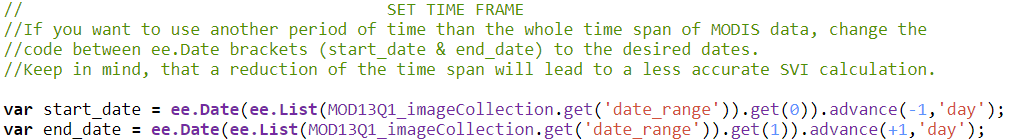
The strengths of the Google Earth Engine lie in the computing power, less so in the export of large image collections. Therefore, a reduction of the images to be exported might be useful. Providing a timescale out of which you would like to download the SVI images will add those images to the "Tasks" tab.
3. Accessing imagery
3.1 GEE ImageCollections
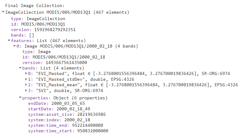
One major advantage of GEE is the accessibility of global time series data in the form of ImageCollections. These are already loaded on Google's servers and do not require much pre-processing. ImageCollections have an ID (e.g. MODIS/006/MOD13Q1) and contain a certain type or quality of data. ImageCollections can be reduced by applying filters on the region, the date of acquisition or other metadata-filters (e.g. cloud-cover). The GEE code provided in this Recommended Practice prints filtered ImageCollections to the console where they can be explored manually.
3.2 Satellite sensor
The enhanced vegetation index (EVI) is used for the calculation of the SVI. The EVI is derived from data captured by MODIS (Moderate-resolution Imaging Spectroradiometer). MODIS is a sensor carried by the Terra and Aqua satellites and delivers data for the EVI in a resolution of 250m.
3.3 Resolution
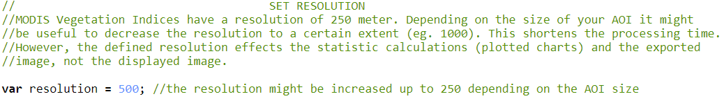
As mentioned above, the MODIS data comes with a resolution of 250m. As the time required to run the calculation increases with an increasing resolution, it might be useful to decrease the processing resolution to a certain extent. The resolution can be modified by the user within the "Set resolution" section in the script. The default value is set to 500m to enable a quick calculation of the demo AOI. The chosen resolution affects the calculation of the mean SVI within the AOI, which is displayed in the charts; it also affects the resolution of the exported images. It does not affect the resolution of the displayed images in the Google Earth Engine.
3.4 Cloud mask
The script features a cloud-and-snow-masking algorithm based on each image's pixel quality assessment band. Thereby, snow and clouds are removed from all images of a collection. The "SummaryQA" band has been used in this script to mask out all pixels with a low quality. A more detailed mask is available for MODIS data (called 'DetailedQA') and can be used to modify the masking algorithm. This mask has not been implemented into the script in order to keep it handy. Skilled users might adapt the script to use the 'DetailedQA' band for the masking process.
4. Obtaining additional information
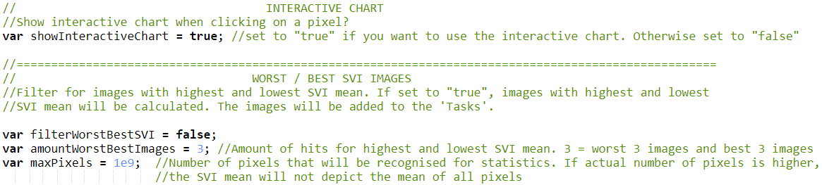
You can activate or deactivate additional features such as the creation of an interactive chart that plots the SVI timeline by clicking on a location in the map-section of the interface or the calculation of the images with the highest and lowest average SVI. The creation of the interactive chart is enabled by default, but can be disabled if desired. The calculation of the images with the highest or lowest average SVI is disabled by default as it needs some time to be executed. Despite the function to enable or disable this feature, you can provide the number of images to be selected for this calculation. For example: enabling this feature and entering the number 3 will result in the calculation of the three images with the highest average SVI and the three images with the lowest average SVI, and add them to the "Tasks" tab for download. However, just the image with the highest and the lowest SVI will be displayed as a layer.
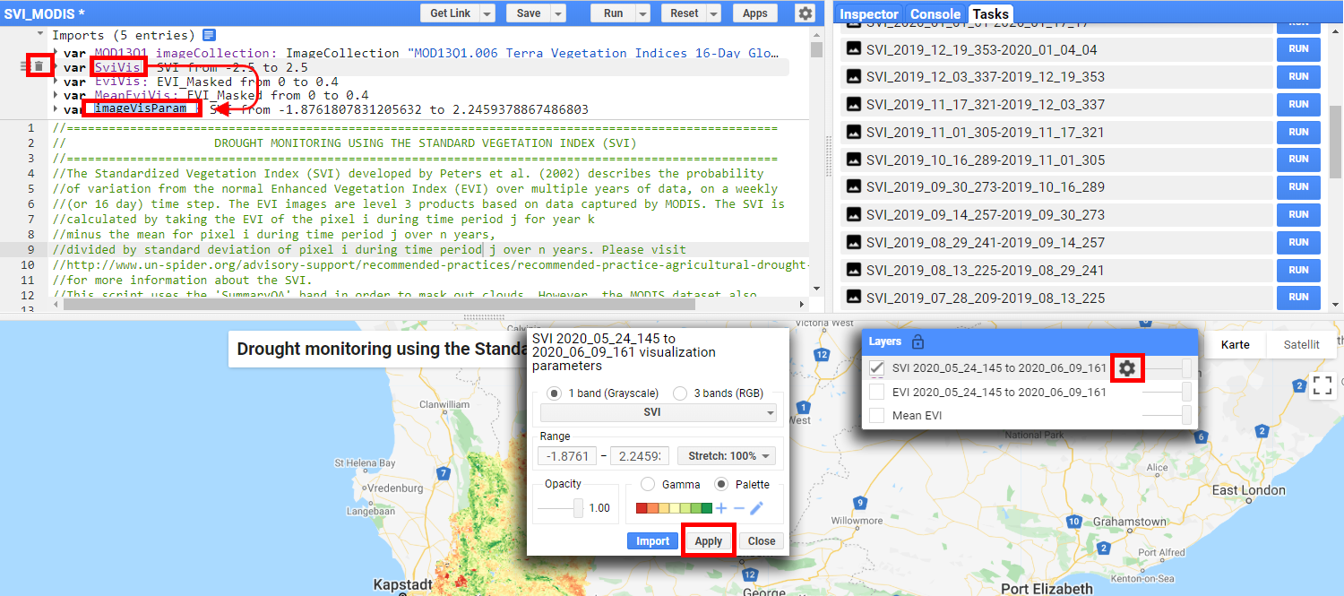
After finishing the calculations, Google Earth Engine will display the latest SVI image in the map section. The latest EVI image and the mean EVI image of the whole timescale will be added to the "Layers", but will be deactivated. You can visualize them by hovering over "Layers" and activating their checkboxes. A visual comparison of the layers can be conducted by using the sliders. In order to receive a pixel value from the visualized images go to the "Inspector" tab and click on a location within you AOI.
The charts, which are printed into the "Console" display the EVI and SVI over time by taking the mean of all pixels in your AOI for each acquisition date. A positive SVI indicates a good vegetation condition which is better than the average for the specific period. A negative SVI indicates a worse vegetation condition compared to the average of the specific period. This phenomenon might be connected to droughts. The severity and spatial distribution of droughts that occurred in the past can be examined by analysing the graphs and the images. Even the observation of imminent droughts might be possible if combined with additional data sources.
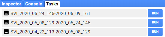
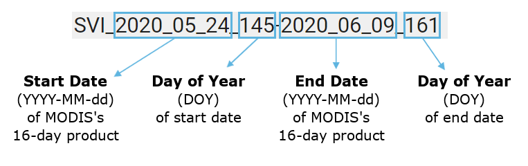
Downloading the results might be inevitable for further analysis. However, as mentioned above, downloading large image timelines is not one of Google Earth Engine's strengths. Should you want to download the images, you can start the download of the images by selecting the "Run" button of each filename within the "Tasks" tab. It is possible to start all tasks at the same time by using this script. The naming of the files follows this scheme:
Limitations
Providing an AOI with a large spatial extent or overly increasing the processing resolution might cause server-based timeouts. An alert might appear to indicate that the website is not responding. You can press "wait" in order to wait until the server finishes the calculations. This might not always solve the problem of processing timeouts. Sometimes a downsizing of the AOI or an increasing of the processing resolution is inevitable.
The legends pick their maximum and minimum values from the visualization parameters in the "Imports" section. If you wish to adapt the numbers in the legend to a new visualization layout, you have to import the new settings to the script, delete the old visualization parameters and rename the new parameters to the same name as the old ones before re-running the script.