1. Band Selection
The S-2 acquire data in 13 spectral bands: four bands at 10 meters, six bands at 20 meters and three bands at 60 meters spatial resolution through Multispectral Instrument (MSI).
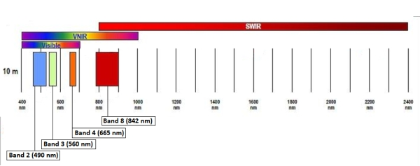
Figure 1: SENTINEL-2 10 m spatial resolution bands: B2(490 nm), B3 (560 nm), B4 (665 nm) and B8 (842 nm)
The bands used for this process are green and near-infrared (NIR) which fall in the 10 meters category. If you want to create a true colour composite you can additionally select the blue and red band. These can be selected and directly imported into QGIS as shown in figure 2.
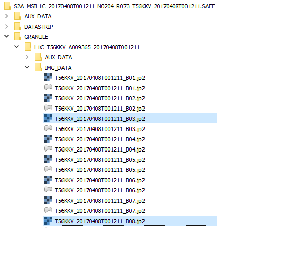
Figure 2: Sentinel 2 Green ("B03") and NIR ("B08") Selection in Layer Browser
1.1 Set the coordinate reference system
Next, set the coordinate reference system by going to properties and selecting the coordinate system WGS84.
And disable "on the fly projection" if this is an option in the Version of QGIS you are using.
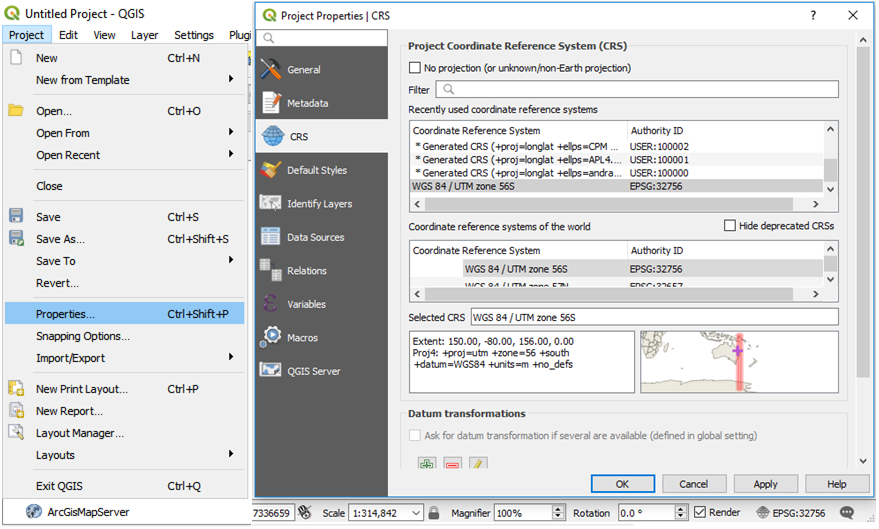
Figure 3: Setting of CSR to WGS84 UTM zone 56S. This zone has the least distortions in Australia.
2. Top of the Atmosphere (TOA) Corrections
The first step before calculating the NDWI is to apply a top of the atmosphere correction in order to get the actual reflectance emitted from the objects on the Earth's surface.
2.1 Installing the Semi-Automatic Classification Plugin
To correct for the TOA in QGIS, the Semi-Automatic Classification plugin is used. So before correcting, please be sure that you have the plugin installed. To install it, please go to Plugins -> Manage and install plugins… . After clicking on Manage and Install Plugins… a new window should open where you can search for plugins to be installed. Please type on the search box 'Semi-Automatic'; after typing it should automatically show you the plugins options that correspond to the search (Figure 4). After selecting the Semi-Automatic Classification (SCP) Plugin, please click install on the bottom right corner of the window (indicated by the red box in Figure 4).
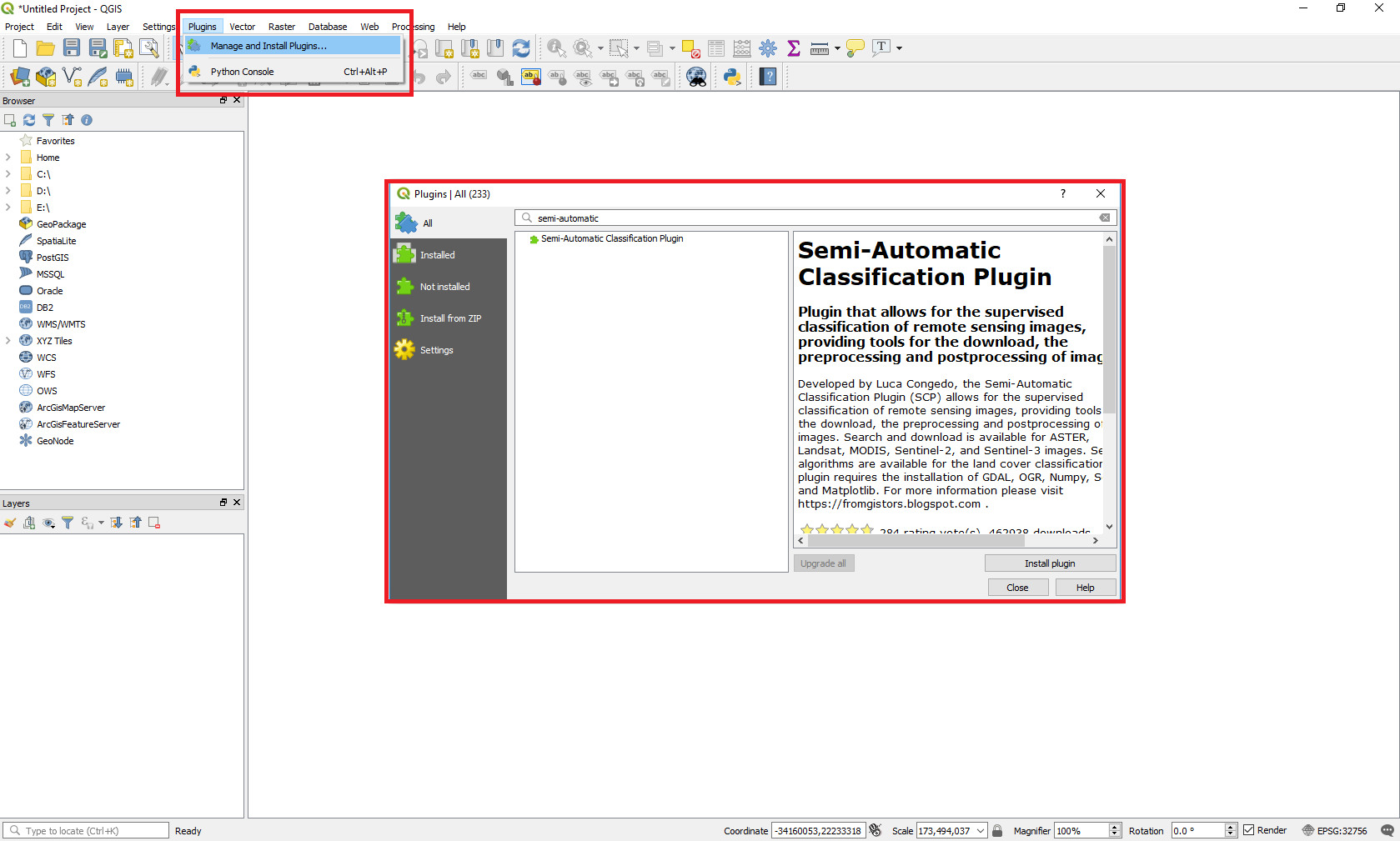
Figure 4: Plugins' search in QGIS
2.2 Top of the Atmosphere (TOA) corrections
So now there should be an SCP icon on your menu toolbar. Please go to SCP -> Preprocessing -> Sentinel-2, as demonstrated in Figure 5.
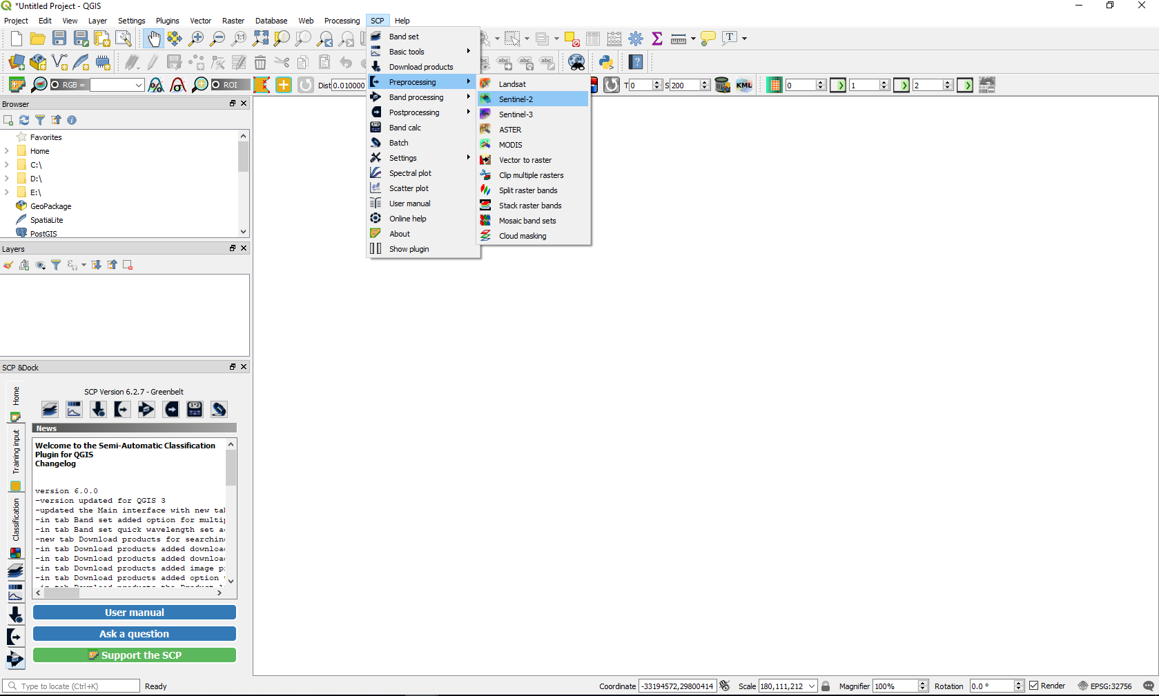
Figure 5: Path to follow to SCP -> Preprocessing -> Sentinel-2
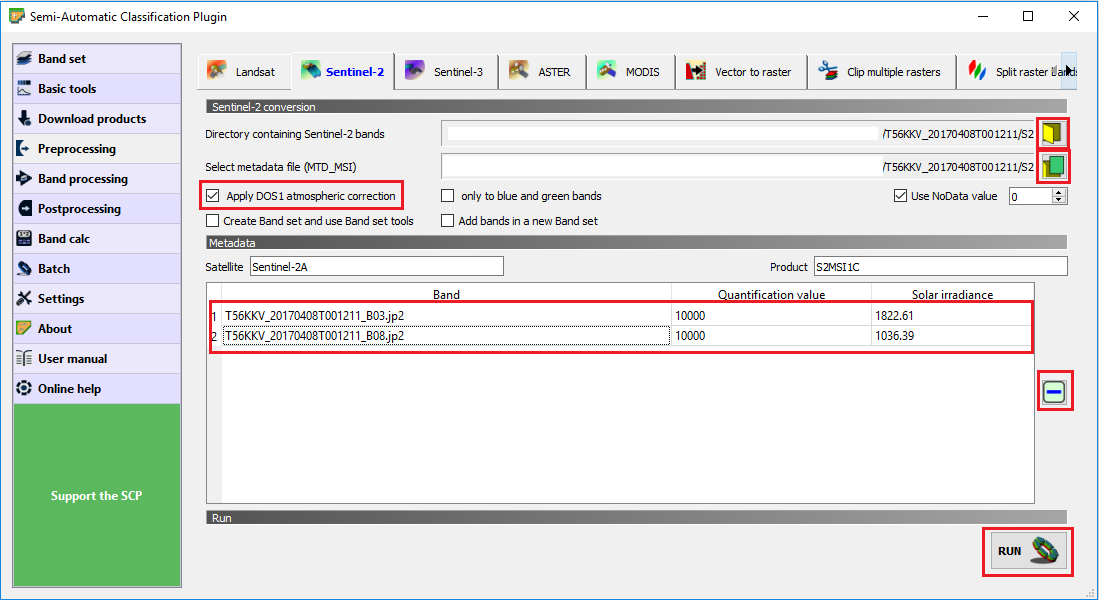
After following the path and clicking Sentinel-2, a new window should open, such as the one shown in Figure 6. Click first on the yellow icon indicated by a red box in Figure 6 to select the folder where your images are and then on the icon below to select the folder where metadata is (file MTD_MSIL1C). After selecting the folder that contains the pre-fire images, you should see your folder path on the 'Directory containing Sentinel-2 bands' and on the 'Select metadata file (MTD_MSIL1C)' and below that you should also see the bands that are in the selected folder. On the SCP processing window, please select Apply DOS1 atmospheric correction. Leave also Use NoData value (image has a black border) option selected. Select the bands that will not be used during the NDWI process and remove them (click the 'minus' icon in the red box indicated in Figure 6 on the right-hand side), i.e. remove all bands except 3 and 8. Finally, click run and it will ask you to select the folder where the corrected images will be stored.
3. Flood Extent Extraction
In order to extract the flood extent, the Normalized Difference Water Index (NDWI) is calculated using the green and near-infrared bands through the following formula in the raster calculator. In this step it is also advised to reduce the extent of the layer to your study area to reduce processing time. After this point clipping the flood to the required extent should only be done after once all shapefiles are complied at the end of step 5. Open the Raster Calculator by clicking on "Raster" > "Raster Calculator". Use select layer extent to focus on the area of interest and enter the expression shown in figure 7:
(Band 3 - Band 8) / (Band 3 + Band 8)
An output layer, here named NDWI, will be produced.
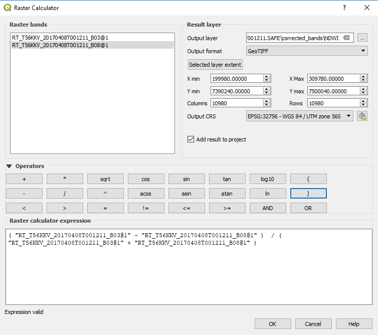
Figure 7: Raster Calculator with NDWI expression
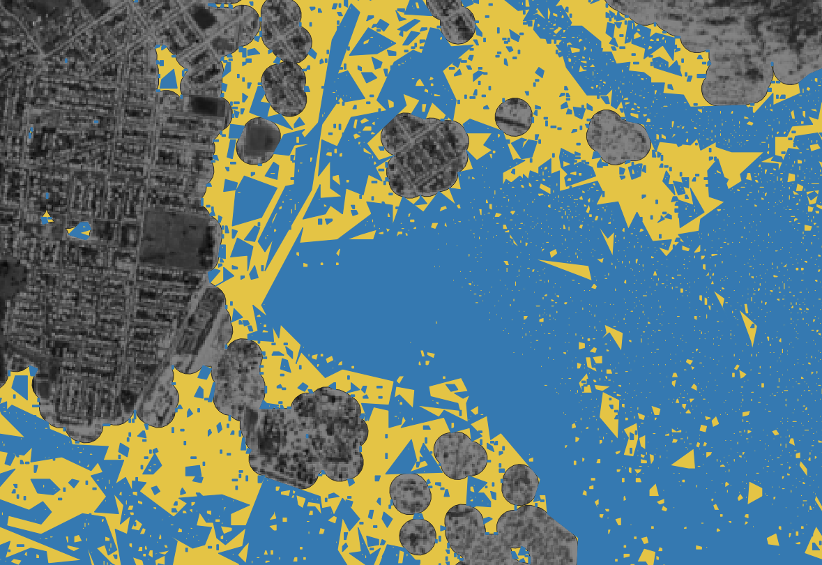
This should yield the following output:
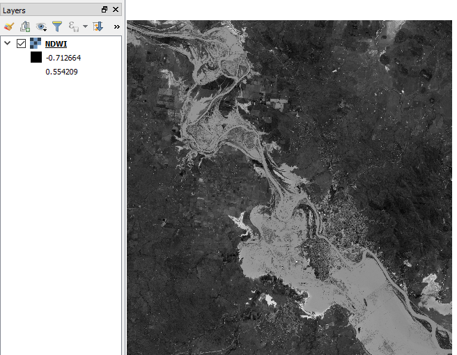
Figure 8: NDWI Output layer
3.1 Binarization
In order to extract the flood outline the NDWI image will need to be binarized. This means that all pixels will be assigned a value of 0 or 1 which corresponds to flood or no flood.
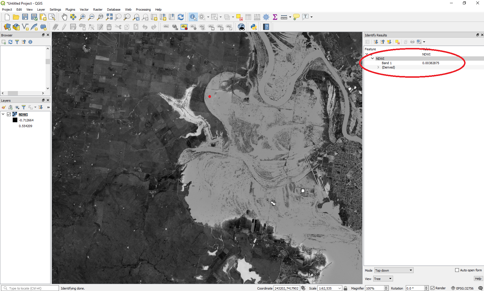
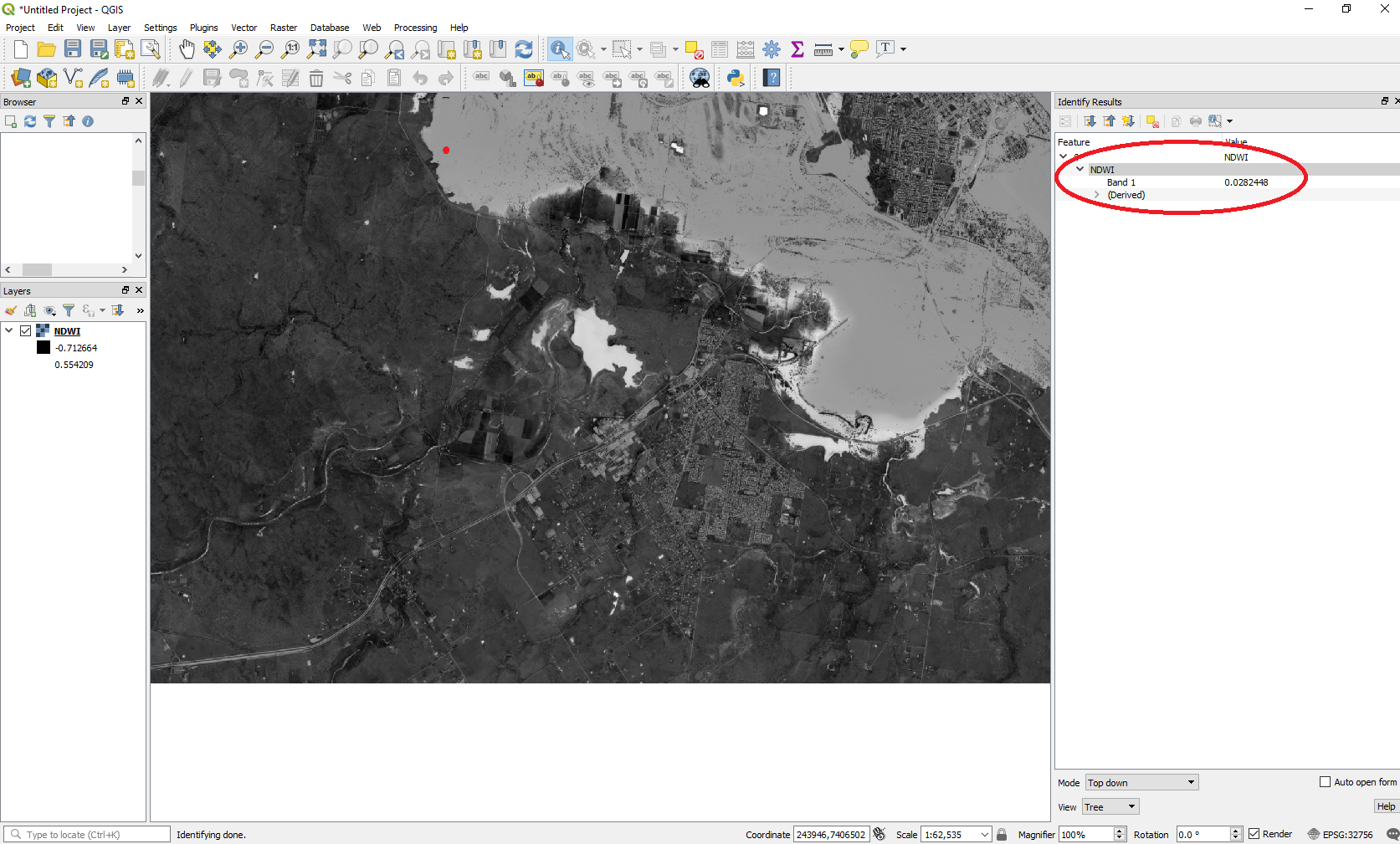
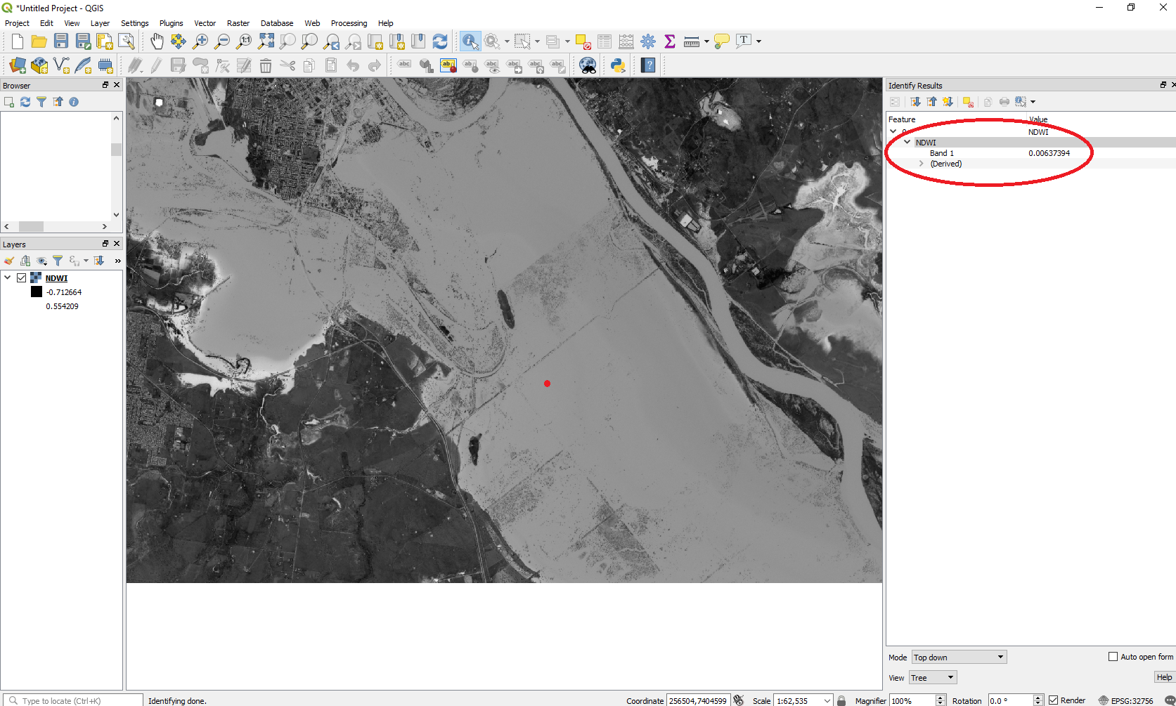
In order to do so, a threshold needs to be identified. This can be done by sampling the digital number values in flooded areas to obtain an average.
Sample 1:
Sample 2:
Sample 3:
Sample 4:
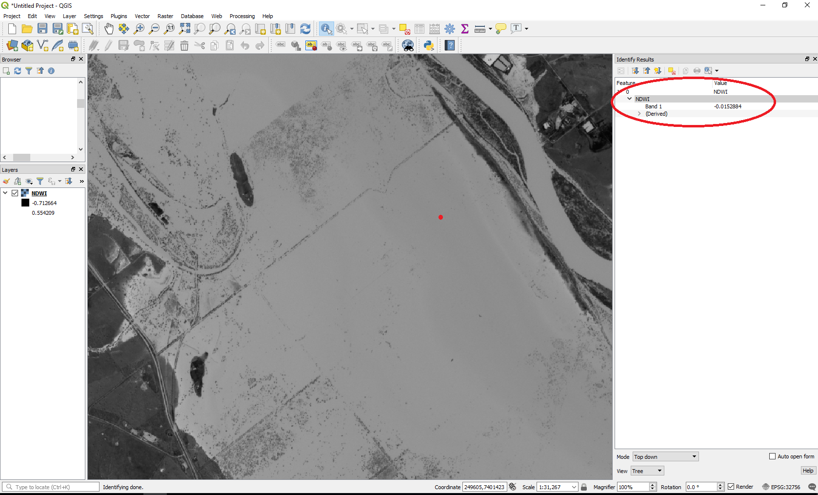
Figure 9: Point samples of NDWI values.
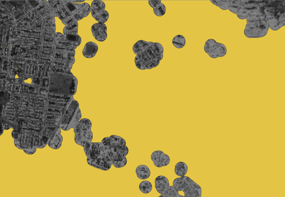
In our case the ideal value was found to be 0.0058. To check whether this is the ideal value the single band can be rendered by assigning the found value in the min and max tab of the symbology field. Click right on the NDWI tiff file in the layers tab and then on "Symbology". If this results in too much noise the value should be readjusted.
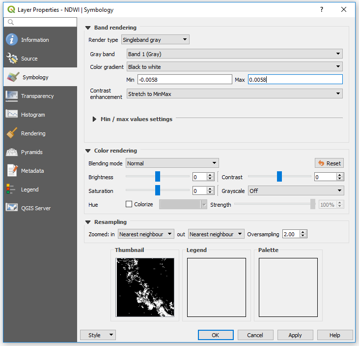
Figure 10: Binarization testing through setting minimum and maximum in the symbology tab.
If you are happy with the found threshold take note of the value and open the raster calculator. Select the NDWI band and use the following expression (NDWI@1 >= X) where X is your threshold to binarize the flood extent (Figure 11). The output of this step will be a binarized tiff.
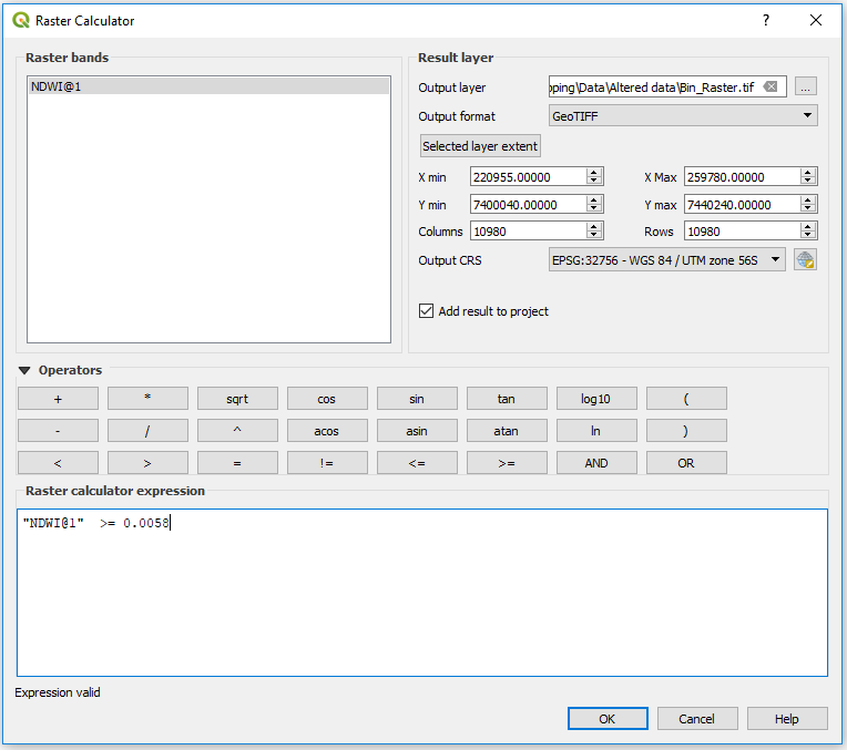
Figure 11: Raster calculator binarization
3.2 Polygonize to Vector
The generated tiff file can now be converted to a vector file. This process is called "Polygonize (Raster-to-Vector)" in QGIS and can be found if you through the menu panel Raster -> Conversion -> Polygonize. The outcome of this process is the shapefile of the flood extent which is used in later steps.
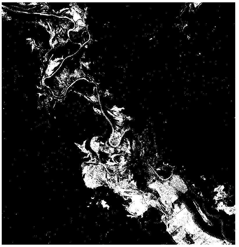
Figure 12: Binarized image
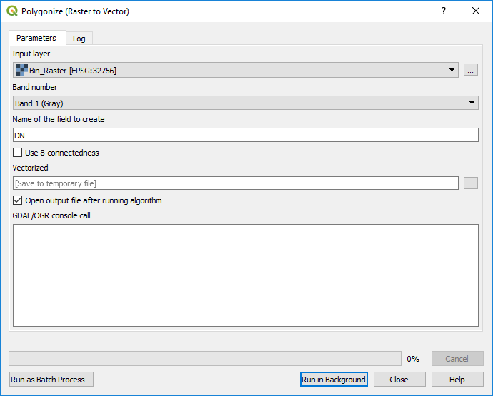
Figure 13: Polygonize Toolbar
The Vector Layer will initially cover the total area. To extract the flood all 0 values need to be deleted. Open the attribute table by right clicking on the vector layer.
Click on toggle  and in the expression bar that appears below type 0 and click "Update All". When the zeros are highlighted click on the red bin item to delete
  . The output should look like figure 14 below.
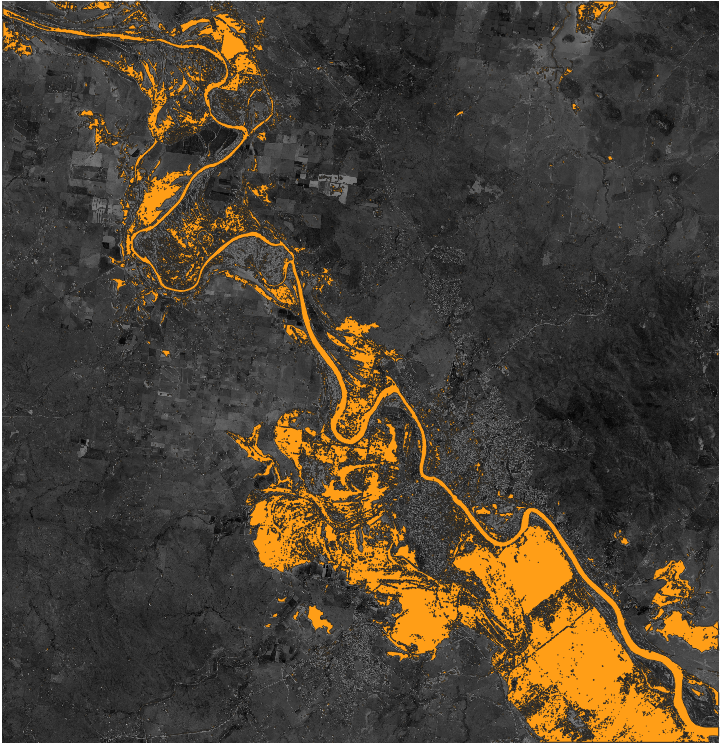
Figure 14: Vector output of the polygonization
3.4. Geometry Fix & CRS setting
Since the shapefile has been created from an image the geometry needs to be fixed and the CSR should be re-defined. This option can, similar to the polygonize function, also be found in the processing toolbox. Once the fix geometry process has run, the shapefile should be exported with the coordinate reference system (CRS) being set.
By right clicking on the fixed geometry layer select the export option and click Save Feature As….
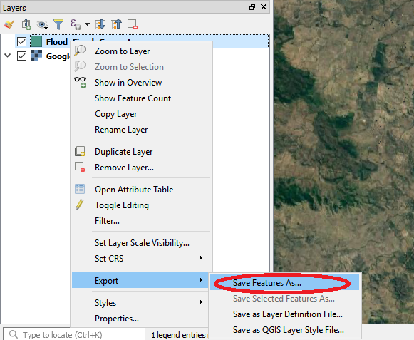
Figure 15: Export vector layer in correct CRS

Figure 16: CRS Selection
Once that field opens select the appropriate CRS for your study area. In our case the appropriate choice is EPSG: 32756. To find out more about the use of coordinate reference systems on QGIS follow the link.
4. Extraction of relevant flood extent
During the polygonization a large number of small polygons are created. These can occur on wet rooftops, wet streets or artificial water bodies such as pools or reservoirs that do not necessarily represent the actual flood extent. The high number of polygons requires long processing times and disturbs the analysis of the effects of the flood we are interested in. It is therefore suggested to clean the flood extent shapefile of these polygons.
First, the main consideration is the method to identify which polygons should be excluded from the analysis. In this case we removed all polygons smaller than 600 sqm, a higher or lower threshold can be chosen as well. This way we can reduce 19’000 features to ~6’000. This was done using the area function in the field calculator. In order to calculate the area, open the field calculator and select "Create a new field". Simply type $area in the Expression tab and click "OK".
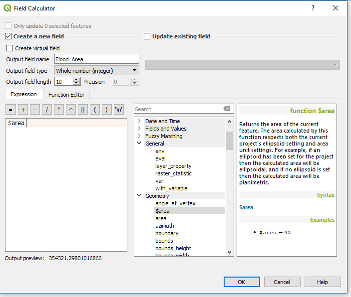
Figure 17: Calculate $area with field calculator.
Next open the "Select by Expression" feature and select all areas under a certain size. You can zoom into what seem to be outlier polygons in your area of interest and see whether they are selected with the size you have chosen and adapt appropriately. The choice of size to exclude polygons affects the accuracy of final results, however, it can significantly improve calculation efficiency. When you are happy with your choice, once again choose toggle and then delete .

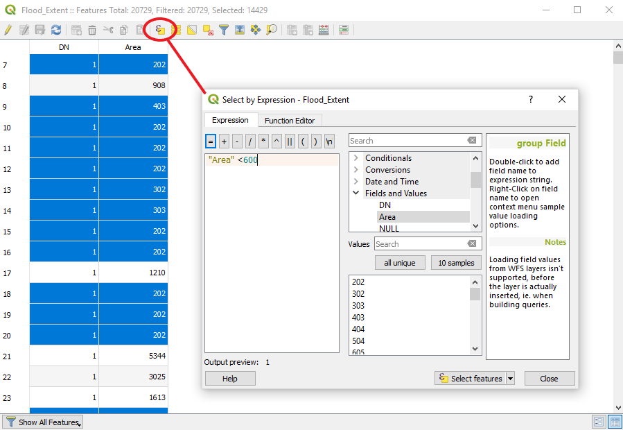
Figure 18: Deletion of all layers smaller than 600 square meters.
Second, since we are only interested in the 2D extent of the flood and not the river, we can make a difference between the flood layer and a vector layer of the river. “Vector overlay > Difference” in the processing toolbox (Ctrl-Alt-T).
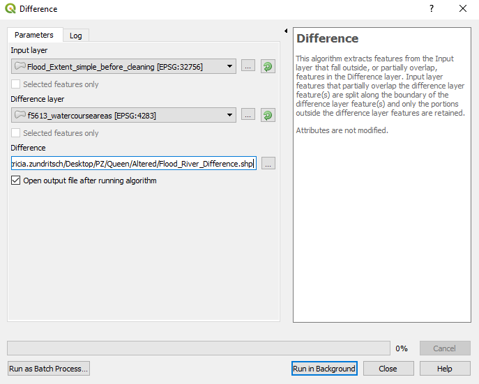
Figure 19: Difference with permanent water body layer
Buffer Processing
Third, we can join all polygons in the immediate vicinity, by adding a buffer off 20m around them, and afterward subtracting it again. To do so, select your flood extent with the "Vector geometry > Buffer Tool” in the processing toolbox, set the buffer to 20m and click dissolve result. Note: if there is a problem with the geometry, apply the tool “Vector geometry > Fix geometries”. After this has run, input your FloodExtent_Buffer into the same tool, setting the Buffer to -20m. By adding the negative sign we will subtract the added area from around the image, but keep the inside of the polygons joined together.
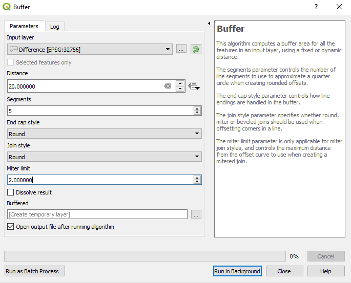
Figure 20: Buffer processes
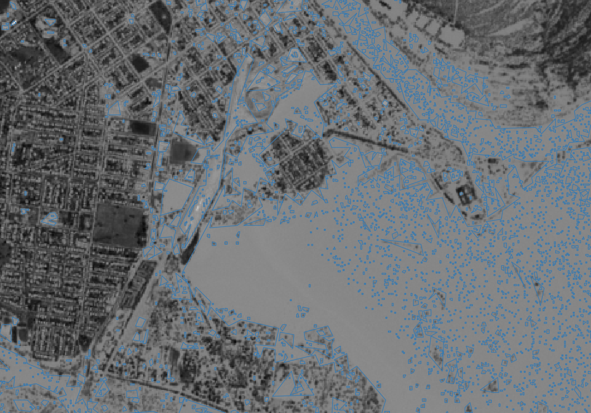
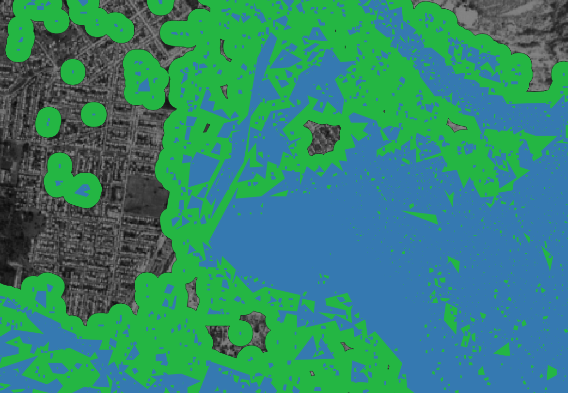
The figure 21 illustrates the effect of the buffer. While initially there may be many small polygons inside larger polygons such as in figure 21. A buffer that simply increases the perimeter of the images and dissolves the features inside, would increase the the size of the flood. This setp is shown in green (Positive buffer +20m). To retract the added surface, the negative buffer in yellow (-20m) illustrates the boundaries of the initial layer (slightly rounded) but with holes inside.
|
|
|
| Initial flood extent vector with "holes" | Figure 21: Buffered flood extent (+20m) |
|
|
|
|
Effect of negative buffer (yellow). Retraction of outerboundaries back to original edges, but filling in holes. |
Flood extent after buffer process |
Since this buffer is meant to join areas inside a polygon that were disconnected on the satellite image, this option can affect the size of the flood (for example if the holes inside the polygon represent streets). With visual verification the buffer size can be set to achieve the best tradeoff between accuracy and ease of computation. Alternatively, polygons can also be smoothed using the simplifying geometry function in the process toolbox before the cleaning processes.
Figure 22: Flood extent after buffer process with transparent style in order to show the satellite image below.
Depending on the study area you might want to alternatively clean up the polygons manually which can be time intensive. A selection of the extent around the main water body can be achieved with the tool “Select by Freehand”. In this way, only larger effects around the main river are studied. Finally, open the attribute table and make sure that there is only one line. If there are still multiple features, go to the tool “Dissolve” and select your layer. Once you are satisfied with the level of detail of your flood extent, save all the shapefiles and close QGIS continue to Step 5.
5. Attributes / Statistic Calculation
In this section, attributes of the affected infrastructure and relevant land use will be calculated through the following procedure. It may be noted here that the inundation layer extracted through the above mentioned procedure can be used as a mask for attributes / statistic calculation.
5.1. Setting CRS & Importing layers
To perform the damage assessment calculation of the affected area open a new project in QGIS. Now set the CSR to the one you selected in step XX and disable the on the fly projection. (Only necessary inQGIS 2.18, in newer versions this is disabled automatically). Then, load your areas of interest such as the inundation area, road, settlements, districts and the imagery (of the desired resolution and band combination) layers into QGIS.
5.2. Select Affected Districts
Then open the tool “Select by location” from the Processing manager on the right. Select from the District polygon those that “intersect” with the simplified flood polygon. This will highlight only the districts we are interested in.
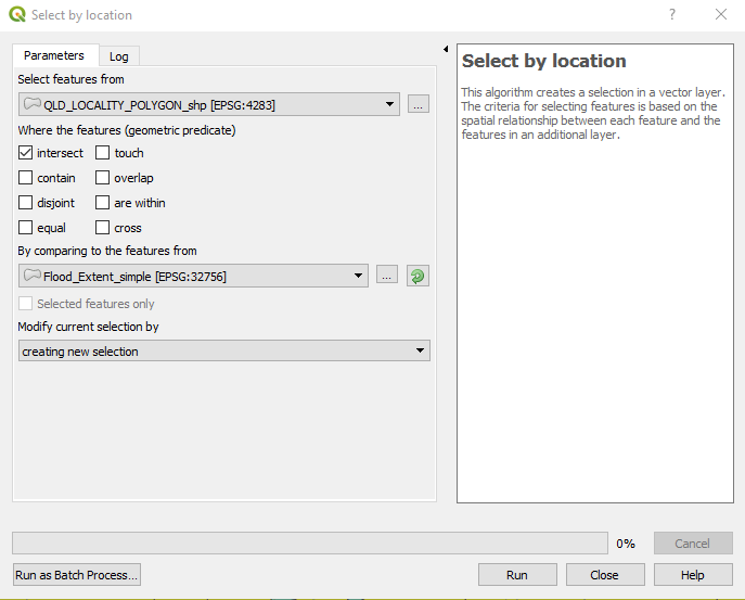
Figure 23: Select flood polygons by districts
Next, save only this selection by right clicking on the ”Intersection” layer in the Layers Tab and selecting “Save as …”. Set your file location and CRS and make sure that the option “Save only selected features” is ticked.
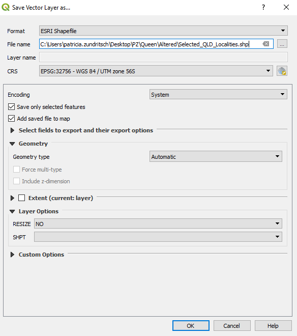
Figure 25: Save only selected features
Finally, if you still have more than one attribute, because you choose not to apply the buffer processing, dissolve the features.
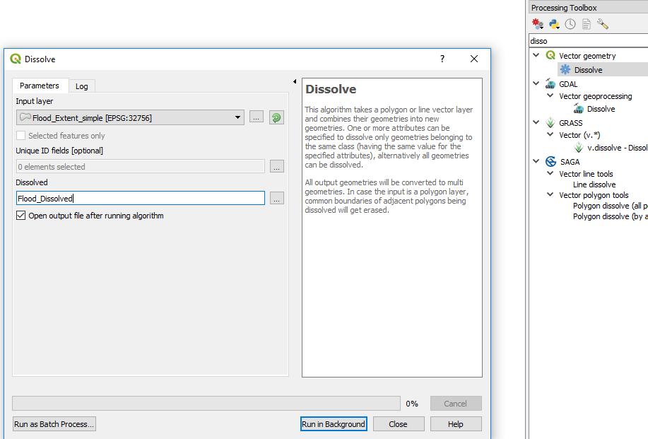
Figure 26: Dissolve all features in one layer
5.3 Intersect District Polygon with Flood Polygon
In order to get district-wise affected inundated areas, open the intersection tool [Processing>Commander: “Intersection”]. Use the final flood extent after cleaning as an input layer and intersect it with the selected districts.
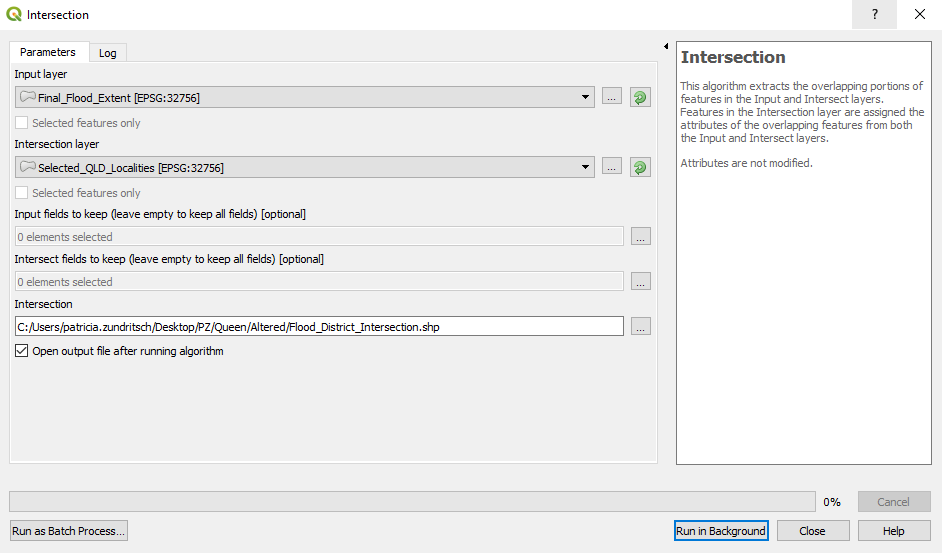
Figure 27: Intersection of flood extent with districts
Check the attribute of the intersected layer [Right click on the desired layer and select attributes]. Delete the old area attribute which is no longer accurate and add a new field. First click  to enable editing, and then select delete field/column. Depending on the attributes layer here, additional cleanup such as deleting columns can be done here as well.
Add a new column “Flood_Area” in the attributes table of the flood in order to calculate the inundation area in sqm. Select a new column and click right, then select field calculator, then add $area from geometry as shown below. >Note: if sqkm are desired the calculation must be “$area/1000000”.
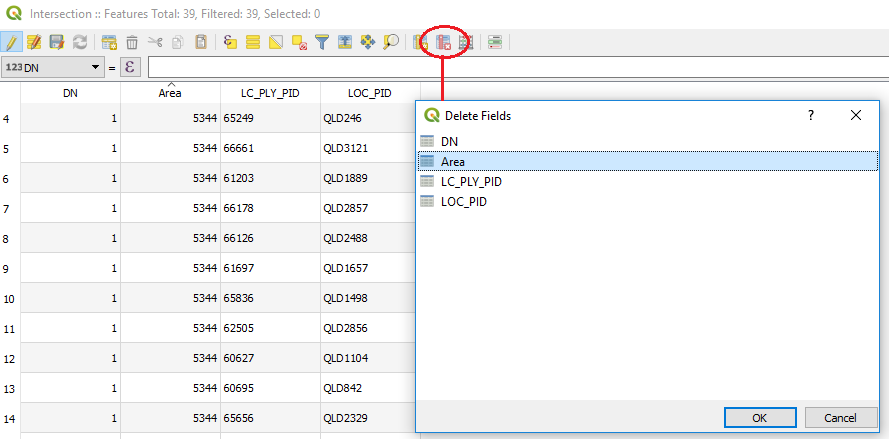
Figure 28: Delete area column in attribute table
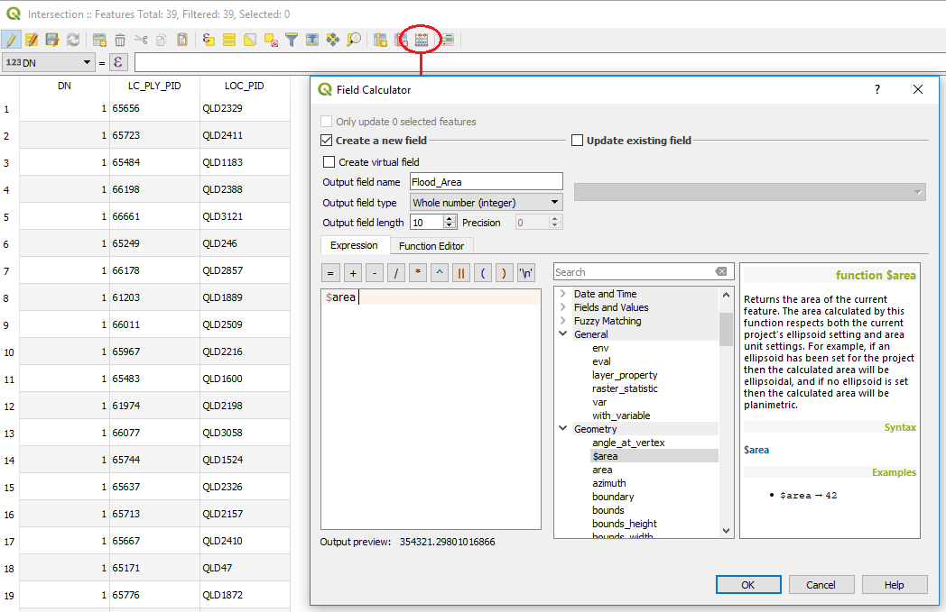
Figure 29: Calculate area of flood by district
5.4 Intersect Road lines with Flood Extent
To extract the affected roads and to be able to map them easily, intersect the Road layer (Input) with the final flood extent. As opposed to the District-Flood Intersection the result is a line layer. The length of affected roads can also be calculated with the field calculator. Simply create a new field and select “$length” to get the road distance in meters or divide by 1000 to get kilometers.
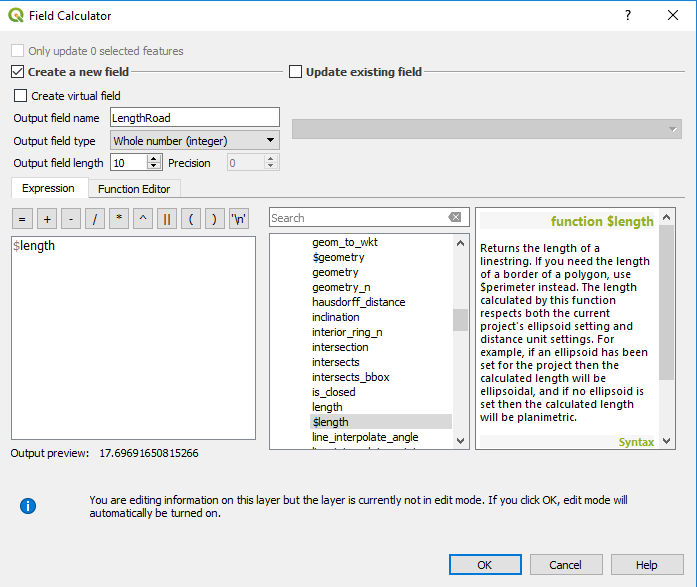
Figure 30: Creation of road length field
5.5 Count Affected Roads and Calculate Road Length
If only the number of roads affected, and the total length per district is needed, 5.5 is not necessary. Using the tool “Vector analysis > Sum line lengths” enter the road line shapefile for the lines and the affected districts polygon as the feature to be summed over.
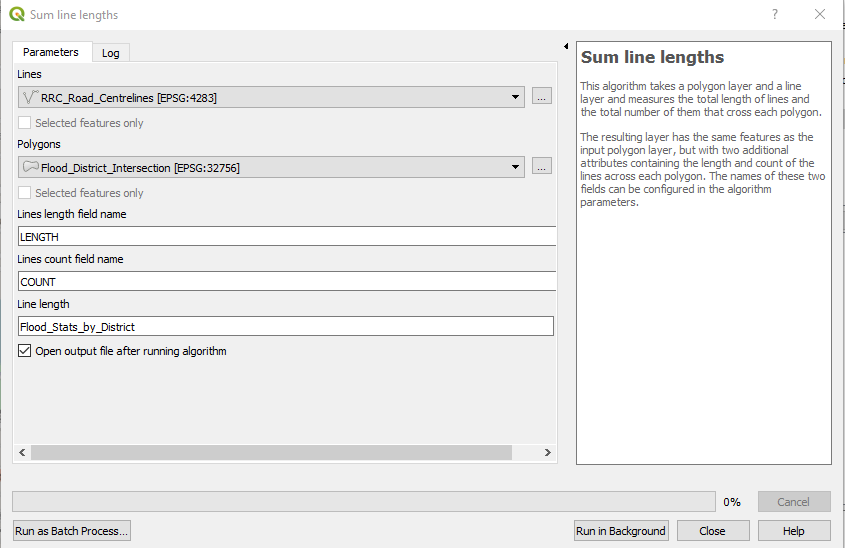
Figure 31: Sum line lengths tool
5.6 Affected Settlements
Load the settlements layer if it has not yet been loaded and make sure that the CRS is the same as for the other project layers. Depending on the region you may have settlements that are polygons or settlements that are points. Working with polygon settlement layers can be facilitated by creating “Centroids” - one point in the middle of each settlement. To do this, search for “Centroids” in the processing commander and select the polygon building layer as input. If you already have a point building layer you can ignore this step.
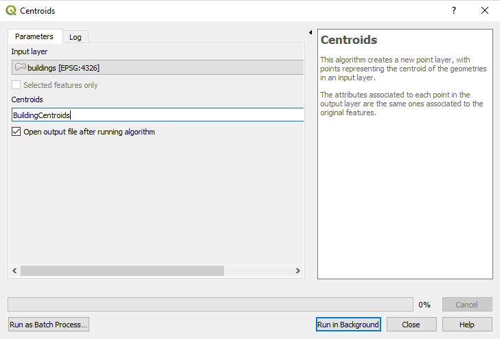
Figure 32: Creation of centroids for polygon settlement layers
Next, use the function “Count point in polygon”, on the District Flood Statistics layer to show how many buildings are affected by the flood. (See page 15) You should find an additional attribute with the number of points for each district flood segment in the Attribute table.
6. Final Output
The final output of this process, is one vector file containing the district wise statistics of the affect or potentially affected infrastructures as well as one vector file of only affected roads. The various information on counts can be illustrated in purely thematic maps to give an overview or joined with the affected roads layer to emphasis emergency locations.
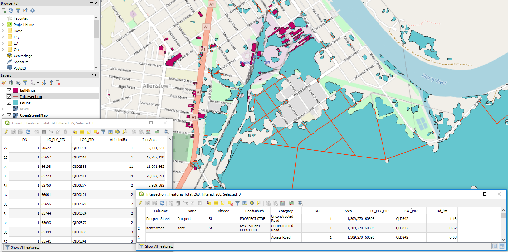
Figure 33: Final output layers